This page collects two projects developed for the Numerical Computing course at Politecnico di Milano. They are presented together as selected academic work: the first project studies the solution of a linear system arising from circuit analysis, while the second moves from Fourier approximation to discrete cosine transforms and image compression.
The source code is available in the two public repositories: Project 1 and Project 2. The original assignment PDFs and supplied input images are kept outside the public repositories.
Project 1: Linear Systems and Iterative Methods
From the Circuit to the Linear System
In the first part I built the mathematical model of a resistor network starting from Kirchhoff's current laws, Ohm's law, and the voltage law on the input loop. The unknowns were 15 internal currents, one input current, and nine nodal voltages, giving 25 unknowns and 25 equations.
After eliminating the branch currents through Ohm's law and substituting them into the node equations, the nodal problem takes the form
The resulting 9 x 9 admittance matrix is symmetric positive definite. This structural property is the important one: by Sylvester's criterion, all leading principal minors are positive, so the LU factorization without pivoting exists and is unique. I also checked strict diagonal dominance by rows and columns, but it does not hold globally; it is therefore not the correct justification in this case.
Direct Methods
I computed the factorization with MATLAB's lu, then solved the two triangular systems using forward and backward substitution. No pivoting was performed, and the solution agreed with MATLAB's A \ b operator:
at the precision used in the computation. This is consistent with the SPD structure of the matrix and with the positive leading principal minors found numerically.
Iterative Methods and Numerical Verification
Starting from the zero vector, with tolerance 1e-11 and at most 1,000 iterations, I compared Jacobi, dynamic gradient, diagonally preconditioned gradient, and conjugate gradient.
- Jacobi converged in 160 iterations. Its iteration matrix had spectral radius
0.8555 < 1, which guarantees convergence for every initial vector. - Dynamic gradient converged in 348 iterations.
- Using
diag(A)as preconditioner reduced the condition number from28.4093to14.7842and the iteration count from 348 to 160. - Conjugate gradient converged in nine iterations, with relative error
3.2587e-16. Since the matrix is SPD and has dimension nine, this agrees with the exact-arithmetic result that conjugate gradient converges in at mostniterations.
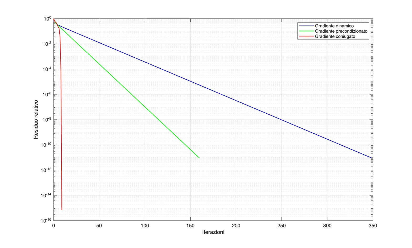
The graph makes the comparison direct: dynamic gradient is the slowest, diagonal preconditioning improves the decay of the residual, and conjugate gradient reaches the tolerance in very few iterations. The observed behavior follows the theory behind the three methods rather than being only an empirical difference.
Project 2: Fourier Approximation, DCT, and Image Compression
Truncated Fourier Series with Composite Simpson Quadrature
I approximated three functions on [0,1] using a Fourier series truncated at maximum frequency n = 15, so the basis has dimension 2n + 1 = 31. I computed the expansion coefficients with a custom composite Simpson implementation.
Composite Simpson quadrature has order four with respect to the subinterval width. For the first two functions I scaled the number of integration subintervals with the sine or cosine frequency being integrated. I then evaluated each approximation on 1,000 points and measured the maximum pointwise difference from the original function.
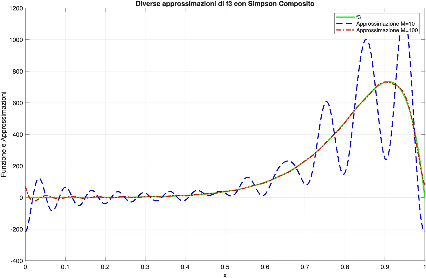
For the third function,
I compared 10 and 100 subintervals. With 10 subintervals, the quadrature is too coarse for the increasingly oscillatory integrands used to compute the Fourier coefficients. With 100, the reconstructed curve closely follows the sampled function in the produced plot.
Custom DCT and Inverse Transform
For the discrete part, I sampled functions at the midpoints of 100 equal subintervals and explicitly constructed the orthonormal DCT matrix D. The one-dimensional transform is the matrix-vector product
and, because D is orthonormal, the inverse is D^T. This also allowed me to truncate the last 60 coefficients of one transformed signal and reconstruct it using the inverse transform, measuring the maximum difference from the original samples.
I implemented the two-dimensional transform by applying the one-dimensional DCT first along the columns and then along the rows:
The corresponding inverse reverses these two changes of basis. The implementation works directly with the constructed transform matrices, which makes the linear-algebra structure explicit.
Performance Comparison
I compared the custom DCT2 implementation with MATLAB's built-in dct2 on random square arrays of increasing size. The plot reports the measurements from that run on a semilogarithmic time axis.
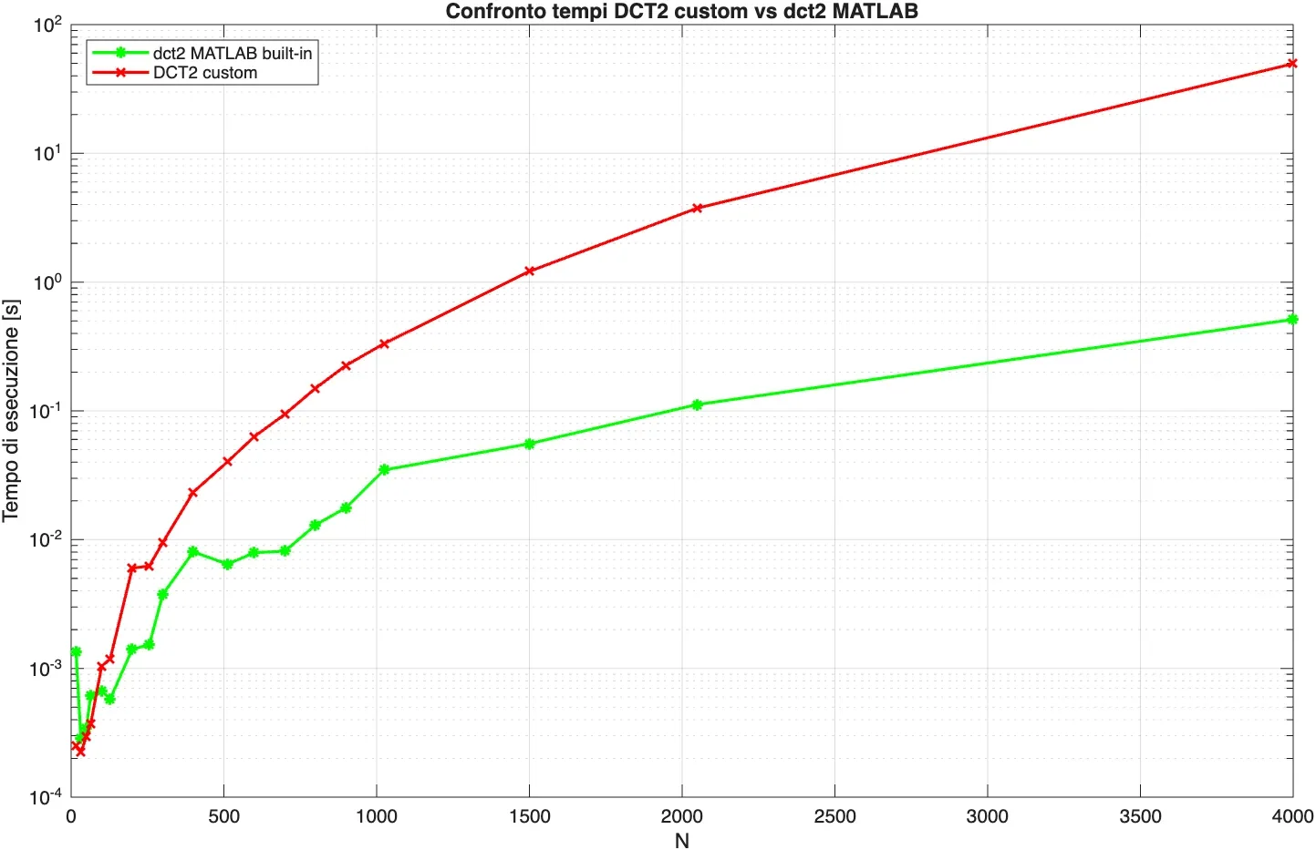
The custom implementation is useful for showing how the two-dimensional transform is assembled, but the measured execution time grows much faster than the optimized MATLAB implementation. The graph is a result of this specific run, not a hardware-independent benchmark.
Block-Based Image Compression
Finally, I used the custom DCT2 and inverse DCT2 to compress grayscale images block by block. For each F x F block, the algorithm:
- computes the two-dimensional DCT;
- sets to zero every coefficient whose indices satisfy
k + l >= dwhen the frequency indices start at zero; - applies the inverse transform;
- rounds and clips the reconstructed pixel values to
[0,255].
Only complete blocks are processed, so any remainder at the image boundaries is discarded. I tested the method on three supplied images with different block sizes and cut-off thresholds, including the deer image with F = 82 and d = 14.
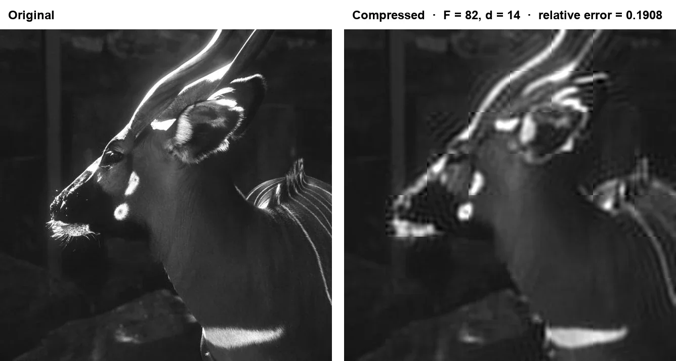
For this reconstruction, the relative Frobenius error is
The visible loss of detail and block boundaries are the consequence of discarding higher-frequency coefficients independently inside each block. The implementation therefore connects the transform, coefficient truncation, inverse reconstruction, and the visual effect of compression in one complete numerical pipeline.