Today I want to explore the breakthrough ideas presented in the paper Breaking the Sorting Barrier for Directed Single-Source Shortest Paths . Before diving into those concepts, it’s important to briefly introduce Dijkstra’s algorithm and its purpose.
1. Introduction: Why SSSP Still Matters
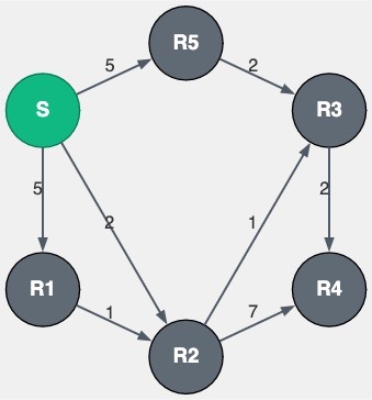
In many practical applications, you work with a directed graph , where represents vertices and the edges. Each edge is often associated with a weight (for our purposes, these must be positive—we will see later why this restriction matters). These weights can model:
- Distances
- Costs of traversal
- Latencies
The fundamental task is to find the shortest path (in terms of total weight) from a given source to all other vertices. This problem is known as the Single-Source Shortest Path (SSSP) problem.
SSSP remains central in many domains, including:
- Routing algorithms in networks
- Networking protocols
- Compiler optimizations
In 1956, Edsger W. Dijkstra devised an elegant solution to this problem. Three years later, he formally published it in his influential paper “A Note on Two Problems in Connexion with Graphs” (1959).
This contribution was historic: it provided a clean and efficient algorithm for a problem that seemed computationally challenging at the time. Given that computers in the 1950s were extremely limited in speed and memory, Dijkstra’s solution was not just clever but fundamental.
Dijkstra’s original form of the algorithm became a cornerstone of computer science. Later decades brought refinements—through improved data structures, heuristic methods, and adaptations for massive graphs—that extended its reach. Yet none have surpassed the foundational impact of Dijkstra’s 1959 publication.
Because of the importance of the SSSP problem, research has continued for decades to improve the time complexity of shortest-path algorithms. And now, after more than sixty years, we have reached a new frontier: breaking the long-standing sorting barrier for directed SSSP.
2. Dijkstra’s Algorithm: The Classical Foundation
In this section, we review how Dijkstra’s algorithm works at a high level. The goal is simple: compute the shortest path from a given source to every other vertex in the graph.
Formally, consider a graph , where is the set of vertices and is the set of edges. Each vertex stores a value , representing its current best-known distance from the source, and a list of its adjacent vertices.
Initialization.
- Set the distance of the source vertex to .
- Set the distance of every other vertex to .
- Maintain a set of processed vertices (conceptually useful, though not always explicit in implementations).
- Maintain a priority structure containing all vertices, keyed by their distance .
Main loop.
While is not empty:
- Extract from the vertex with the smallest .
- Add to .
- For each adjacent vertex of , perform a relaxation step: update ’s distance if the path through is shorter than its current value.
Relaxation means checking whether:
and, if so, updating .
Pseudocode:
Dijkstra(G,source):
    Initialize-Graph(G, source)
    S = EmptyList()
    Q = List(all vertices in G)

    while Q is not empty:
        u = ExtractMin(Q)
        S.append(u)
        for each vertex v adjacent to u:
            Relax(u, v)
Because the algorithm always chooses the vertex with the smallest distance, it is classified as a greedy algorithm. Greedy methods do not always guarantee correctness in general, but in this case correctness can be formally proved using induction on the size of .
Complexity. In Dijkstra’s original implementation, the priority structure was simply an array. Extracting the minimum then required scanning the entire array, which costs per operation. Since every vertex must be extracted once, this contributes
The inner relaxation loop processes each edge at most once, costing .
Thus, the overall complexity is:
3. Variants and Data Structures: Pushing the Boundaries
The bottleneck in Dijkstra’s original implementation is the Extract-Min operation: finding the vertex with the smallest tentative distance. Using a simple array makes this which quickly dominates runtime on larger graphs.
A major breakthrough came with the introduction of binary heaps as the priority queue for (widely popularized in the 1970s). With this change:
- Extract-Min takes .
- Each edge relaxation may trigger a Decrease-Key, also .
- The overall running time becomes (often written as ), a dramatic improvement for sparse graphs.
On the theoretical side, Fibonacci heaps (Fredman & Tarjan, 1984) pushed the asymptotics even further: . Here, Decrease-Key runs in amortized . While elegant in theory, Fibonacci heaps are rarely used in practice because of pointer-heavy structures, large constant factors, and poor cache performance. This highlights a recurring lesson in algorithms: asymptotic optimality does not always translate into real-world efficiency.
For graphs with bounded integer weights, an alternative approach is Dial’s algorithm (1969). It uses an array of buckets indexed by distance values, achieving: where is the maximum edge weight. On road networks or latency graphs with small integer costs, this method can be extremely efficient.
Other heap structures — pairing heaps, radix heaps, relaxed heaps — have been proposed over the years, each balancing theoretical guarantees and practical constants in different ways. Yet despite decades of improvements, progress has always seemed tethered to the same barrier: the cost of sorting-like operations lurking inside priority queue management.
4. The New Paper: Breaking the Sorting Barrier for Single-Source Shortest Paths
The 2025 paper Breaking the Sorting Barrier for Directed Single-Source Shortest Paths by Ran et al. presents the first deterministic algorithm that beats the classical:
bound for directed SSSP with nonnegative real weights in the comparison–addition model. It is important to state explicitly that the result holds in this model, since it rules out shortcuts that rely on specialized data structures or RAM-model tricks.
Their result achieves:
This is not a wholesale replacement for Dijkstra’s algorithm. If you require the full ordering of vertices by distance, Dijkstra remains optimal. If you only need the distance values themselves, the long-assumed “sorting barrier” is not inherent.
The analysis assumes two standard technical moves: (i) a degree-reduction transformation so every vertex has constant in/out degree, and (ii) a lexicographic tie-breaking rule so that every path has a unique length. Both are common but necessary for the recursion to work cleanly.
Key idea: shrinking the frontier
The bottleneck in Dijkstra’s algorithm is maintaining a strict total order over a frontier of tentative vertices.
At times this frontier can be size , forcing work for each extract-min.
That’s where the extra factor comes from.
The new algorithm avoids this by working in bands .
Suppose all vertices with are complete, and let be the current frontier of vertices with tentative distances in .
Define the covered set:
Every unfinished vertex with lies in .
Now, depending on the size of relative to , the algorithm takes one of two actions, controlled by a parameter :
- Bulk progress. If , a bounded multi-source shortest path (BMSSP) call finalizes all vertices in with in one shot.
- Frontier reduction. Otherwise, perform rounds of relaxations from . Vertices whose shortest paths use fewer than frontier vertices are finalized.
The remaining ones each select a pivot in ; the number of pivots is at most .
This shrinks the frontier by a factor of about .
In either case, progress is guaranteed: either a large batch of vertices is finalized, or the frontier becomes much smaller.
Parameter balancing and complexity
The performance of the recursion depends on two parameters:
The parameter determines how aggressively the frontier can be reduced in the pivoting step. In the worst case, the number of pivots introduced in one round is bounded by , which contracts the frontier by a factor of . The parameter specifies the band width , and hence the distance threshold within which the bounded multi-source shortest path (BMSSP) subroutine operates.
The recursion proceeds in layers: each layer either finalizes a large fraction of via BMSSP or reduces the frontier by a factor of about . Since the frontier shrinks by in a reduction step, the number of recursive levels is at most
Within each level, every edge is relaxed at most once, and the per-vertex overhead due to frontier reduction is bounded by
Combining these observations, the overall running time is
The balance between and is crucial: larger accelerates frontier reduction but increases per-level cost, while larger decreases recursion depth but inflates the band width and the work of BMSSP. The chosen values and minimize the total overhead and yield the factor.
Runtime comparison
| Algorithm | Time complexity | Applicability |
|---|---|---|
| Dijkstra (array) | Historical baseline; easy to implement but quadratic on large graphs | |
| Dijkstra (binary heap) | Standard practical choice; efficient for sparse graphs and widely deployed | |
| Ran et al. (2025) | First deterministic algorithm to beat the bound in the comparison–addition model |
The 2025 result is not a practical replacement for heap-based Dijkstra. Its significance lies in theory: it shows that the factor in SSSP is not inherent. The breakthrough is stated in the comparison–addition model, where algorithms are only allowed to compare and add edge weights. This model is the standard baseline for analyzing general-weight graph algorithms, since it rules out shortcuts that depend on specialized word-RAM techniques or bounded integers. Citing it makes clear that the improvement holds in the broadest, most widely accepted setting—directly comparable to Dijkstra’s classical bound.
5. Conclusion and Sources
The single-source shortest path problem has been studied for almost seventy years, from Dijkstra’s elegant algorithm to heap-based improvements and practical variants like Dial’s method. For decades, every faster deterministic algorithm seemed shackled by the same bottleneck: the cost of maintaining a sorted frontier.
Ran et al. (2025) show that this barrier is not inherent. By sidestepping the need for a global order and instead settling vertices in controlled batches, their algorithm replaces the overhead with . This marks the first deterministic improvement to Dijkstra’s runtime in the comparison–addition model.
The breakthrough is not just about speed—it’s about perspective. Shortest paths can be computed without ever maintaining a total order of tentative distances, reshaping how we think about the greedy structure of SSSP and opening doors to further refinements.
I hope you enjoyed the post and that it gave you a grasp of SSSP algorithms!
Sources and Further Reading
- Edsger W. Dijkstra (1959). A Note on Two Problems in Connexion with Graphs. Numerische Mathematik, 1:269–271. The original publication of Dijkstra’s algorithm.
- Wikipedia: Dijkstra’s Algorithm. A solid high-level overview with links to variants.
- Thomas H. Cormen, Charles E. Leiserson, Ronald L. Rivest, Clifford Stein (2009). Introduction to Algorithms, 3rd ed.
- Steven S. Skiena (2008). The Algorithm Design Manual, 2nd ed. Emphasizes practical aspects of graph algorithms.
- Ran et al. (2025). Breaking the Sorting Barrier for Directed Single-Source Shortest Paths. The breakthrough paper itself—technical but rewarding for anyone who wants to see the new algorithm in detail.