From Bigrams to Neural Networks: The First Step in Language Modeling

1. Motivation & Goals

In this post, we tackle one of the most fundamental problems in natural language processing: language modeling. Our concrete objective is to build a system that generates plausible Italian names by predicting the next character given the previous one.

Language modeling assigns probabilities to token sequences by predicting the next token given its context. This simple idea underpins tools as familiar as autocomplete and as powerful as large-scale generative models.

We begin with the bigram model: $P(x_t \mid x_{t-1}).$ This model looks back exactly one step, capturing only immediate dependencies. Despite its simplicity, bigrams marked an early step beyond rule-based formal grammars.

From there, we reformulate the bigram as a neural network. This isn’t just reimplementation for its own sake: it shows how fixed statistical tables can be generalized into trainable systems, the very principle that scales into today’s large language models.

With the goal defined, we’re ready to start from the basics.

2. Dataset & Preprocessing

We start from data: the ISTAT list of Italian given names. The raw text contains diacritics, apostrophes, hyphens, spaces, and mixed case. To make the first model tractable, we project the text to a reduced alphabet and remove extremely short items. Formally, we apply a mapping $\phi : \Sigma_{\text{raw}} \;\to\; \Sigma_{\text{ascii}} = \{a, \ldots, z\}$ by lowercasing, Unicode-normalizing, and stripping non-letters; the model is trained on $\phi(\text{names})$.

Normalization choices (trade-offs):

1. Lowercase to collapse case variants.
2. Diacritics → base letters via Unicode decomposition (e.g., Niccolò → niccolo). This shrinks the vocabulary and speeds up training, at the cost of losing some orthographic distinctions.
3. Drop very short names (len < 3) to reduce degenerate contexts and stabilize bigram counts.

Minimal, deterministic preprocessing:

import re

with open("italian_names.txt", "r", encoding="utf-8") as f:
    names = [line.strip().lower() for line in f if line.strip()]

def normalize(name):
    # keep only letters a–z
    return re.sub(r'[^a-z]', '', name)

# Clean and filter
names = [n for n in (normalize(name) for name in names) if len(n) >= 3]
names = list(set(names)) #Now we have a set of uniques names

After preprocessing, we are left with around 15,000 names, which is plenty of data to estimate bigram statistics and to train our first simple models.

3. Vocabulary & Tokenization

Tokens are the atomic units of a language model. In this project, each character is a token, so the vocabulary is simply the set of unique letters in the preprocessed dataset. To handle sequences cleanly, we extend this set with two boundary markers: ! for start-of-sequence (SOS) and ? for end-of-sequence (EOS). Formally, we construct a bijection

and its inverse itos. Encoding applies stoi elementwise to a string; decoding applies itos to a list of indices. Here’s the code:

# Build character set from dataset
characters = sorted(set("".join(names)))

# Define special tokens first 
stoi = {"!": 0}  # SOS
for i, ch in enumerate(characters, start=1):
    stoi[ch] = i
stoi["?"] = len(stoi)  # EOS

itos = {i: ch for ch, i in stoi.items()}
vocab_size = len(stoi)
print(f"Vocabulary size: {vocab_size}")

To illustrate how encoding and decoding work with these mappings, consider the example of the name "tommaso":

name = "!tommaso?"

# Encode: convert each character to its index
encoded = [stoi[ch] for ch in name]
print("Encoded:", encoded)

# Decode: convert indices back to characters
decoded = ''.join([itos[ix] for ix in encoded])
print("Decoded:", decoded)

The output will be:

Encoded: [0, 20, 15, 13, 13, 1, 19, 15, 27]
Decoded: !tommaso?

This mapping turns text into a numerical sequence and back again. By inserting SOS and EOS during training, the model learns both when names start and when they should stop — essential for generating coherent results.

4. Creation of the Training and Test Sets

To evaluate a model fairly, we split the dataset into disjoint parts: a training set to fit parameters and a test set to measure generalization. For this experiment, we use an 80/20 split. Larger projects often add a separate validation set for hyperparameter tuning, but two splits suffice here. Formally, each name is converted into a sequence of pairs $(X_t, Y_t)$, where

Each pair encodes the prediction task: “given the current character, predict the next one.” Implementation in PyTorch:

import torch, random

def create_dataset(names, block_size=1):
    X, Y = [], []
    for name in names:
        prev_ix = stoi["!"]  # SOS
        for ch in name + "?":  # append EOS
            ix = stoi[ch]
            X.append(prev_ix)
            Y.append(ix)
            prev_ix = ix
    return torch.tensor(X, dtype=torch.long), torch.tensor(Y, dtype=torch.long)

# Train/test split 
names_shuffled = names[:]
random.shuffle(names_shuffled)

split_idx = int(0.8 * len(names_shuffled))
Xtr, Ytr = create_dataset(names_shuffled[:split_idx])
Xtst, Ytst = create_dataset(names_shuffled[split_idx:])

At this point, we have compact tensor representations of the training and test data, ready to be fed into the bigram model. To make this concrete, let’s look at how the name "tommaso" is represented:

X, Y = create_dataset(["tommaso"])
for i in range(len(X)):
    print(itos[X[i].item()], "-->", itos[Y[i].item()])

Output:

! --> t
t --> o
o --> m
m --> m
m --> a
a --> s
s --> o
o --> ?

This example illustrates the idea: each pair $(X, Y)$ captures a step in the sequence, mapping the current character (or $\text{SOS}$ at the start) to the next one. The final transition predicts $\text{EOS}$, teaching the model when to stop generating.

5. From Counts to Probabilities

With the training pairs in hand, we can now estimate conditional probabilities. The first step is to build a $V \times V$ count matrix, where $V$ is the vocabulary size and

This matrix encodes the immediate statistical structure of the dataset. By maximum likelihood estimation (MLE) for a categorical distribution:

Intuitively, the chance of seeing $j$ after $i$ is just its observed frequency.

Counting Character Transitions

# Bigram counts matrix: V x V where C[i, j] = times char j follows char i
counts = torch.zeros(len(itos), len(itos))

for i, j in zip(Xtr, Ytr):
    counts[i][j] += 1

# Add-one smoothing to avoid zero probabilities ([additive smoothing](https://en.wikipedia.org/wiki/Additive_smoothing))
counts += 1

Resulting counts (heatmap visualization):

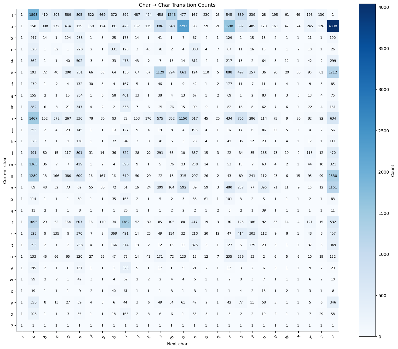
The counts heatmap shows raw transition frequencies: brighter cells indicate more common bigrams (row = current character, column = next character, i.e. row $i$, column $j$ corresponds to $C[i,j]$).

Converting Counts to Probabilities

# Normalize each row to sum to 1
probs = counts / counts.sum(1, keepdim=True)

Each row of probs is a categorical distribution over the next token, and Laplace smoothing ensures even rare contexts yield valid probabilities. Final probability distribution(heatmap visualization):

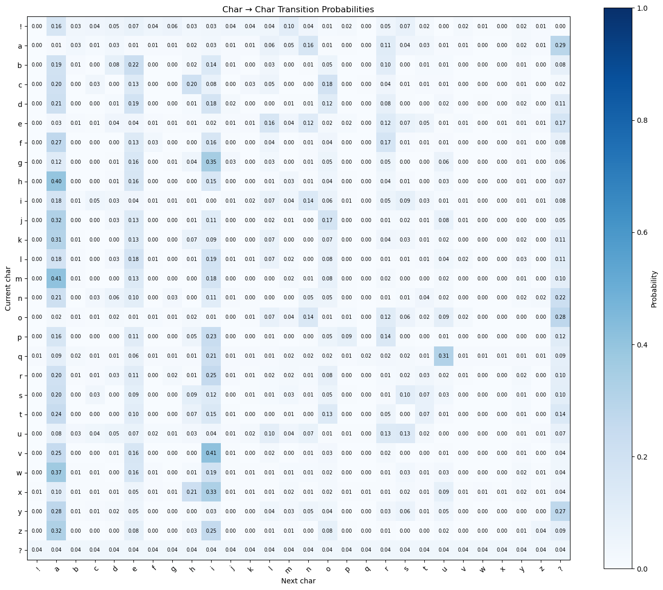
The probability heatmap shows per-row normalized transitions: each row sums to 1, highlighting the most likely successors for every character.

Sampling from the Bigram Model

Now that we have probabilities, we can sample new names. The procedure is:

1. Start with the SOS token (!).
2. Retrieve the probability distribution for the next character.
3. Sample from it using torch.multinomial.
4. Append the sampled character and update the context.
5. Stop when EOS (?) is reached or a maximum length is exceeded.

def generate(n_samples, maxlen=15):
    for _ in range(n_samples):
        context = 0  # SOS
        s = ""
        for _ in range(maxlen):
            prob = probs[context]         # distribution over next char
            idx = torch.multinomial(prob, 1).item()
            context = idx
            ch = itos[idx]
            if ch == "?":
                break
            s += ch
        print(s)

Example Output:

eli
dafo
ada
haariva
anna
minla
gila
coud

Most outputs are noisy or unrealistic, which is expected: the bigram model can only capture relationships between adjacent characters. Still, some generated names look plausible, such as:

• eli
• anna

This shows the model has picked up some local character patterns, but it fails to capture longer-range dependencies needed for realistic names.

A natural idea is to extend the context, e.g., moving from bigrams to trigrams. But this quickly becomes impractical: the size of the count matrix scales as $O(V^n)$, growing polynomially with $V$ and exponentially with $n$, and probabilities become sparse as context length increases. The true solution lies in a different direction — neural networks, which we will explore in the next section.

6. Neural View of the Model

The bigram model was just a lookup table of observed transitions. A neural model reframes this idea as a trainable function.

The setup is unchanged: given a context (initially one previous character), the model predicts the next one. The difference is representation. Instead of fixed rows in a matrix, we introduce embeddings: a learnable map

which assigns each token index a vector in a $d$-dimensional continuous space.

Architecture sketch:

1. Input: previous character index.
2. Embedding layer: lookup dense vector.
3. Linear layer: transform vector to logits
4. ReLU activation: adds nonlinearity, breaking equivalence with a pure lookup table.
5. Softmax: converts logits into probabilities.

Linear Transformation and Nonlinearity

After retrieving an embedding vector for the input token, the next step is to transform it into a representation that can be compared against every possible output class. This is done through a linear transformation:

$z = W x + b$

where

• $x \in \mathbb{R}^d$ is the embedding of the current token,
• $W \in \mathbb{R}^{V \times d}$ is a weight matrix mapping the $d$-dimensional embedding space to the $V$ output classes,
• $b \in \mathbb{R}^V$ is a bias vector, and
• $z \in \mathbb{R}^V$ are the resulting logits, one score for each vocabulary item.

This step assigns a learnable score to each possible next token.

Why Nonlinearity?

If the model consisted only of embeddings and a single linear transformation, it would still be a linear function of the input indices. In fact, a single linear layer is mathematically equivalent to a lookup table — expressive enough for bigrams, but fundamentally limited. With one-hot input vectors, a linear transformation $W x$ just selects a row of $W$. This is functionally identical to table lookup. Only nonlinearities break this equivalence.

To break this limitation, we introduce a nonlinear activation function between layers. In practice, we use the ReLU (Rectified Linear Unit):

$\text{ReLU}(z) = \max(0, z)$

ReLU has two critical effects:

1. It allows the model to compose multiple linear layers into a genuinely nonlinear function, greatly expanding its representational capacity.
2. It zeroes negative activations, which can induce sparse intermediate representations and often improves optimization stability.

Together, the linear layer provides a weighted combination of input features, while the nonlinearity ensures the model is not just a rescaled lookup table. This combination forms the backbone of neural networks and prepares the logits for conversion into probabilities via the softmax function.

The Role of Softmax

The linear layer produces a vector of real-valued scores, or logits, one per token in the vocabulary. These scores are not probabilities. To turn them into a distribution, we apply the softmax function:

where $z \in \mathbb{R}^V$ is the logits vector and $V$ is the vocabulary size.

Softmax has three key properties:

• All outputs are non-negative.
• The outputs sum to 1, yielding a valid probability distribution.
• The exponential transformation sharpens differences, amplifying the highest scores.

Cross-Entropy Loss and Maximum Likelihood

At a statistical level, we assume the data is generated by an unknown distribution $P_{\text{data}}$ over classes $\{1, \dots, V\}$. We define a parametric model $P_\theta$, with parameters $\theta$, that assigns probabilities to these classes. Training aims to choose $\theta$ so that $P_\theta$ approximates $P_{\text{data}}$ as closely as possible.

Maximum Likelihood Estimation

The principle of maximum likelihood estimation (MLE) chooses $\theta$ to maximize the probability of the observed data. Given observations $\{y^{(1)}, \dots, y^{(N)}\}$:

The MLE estimator is:

Negative Log-Likelihood and Cross-Entropy

Maximizing log-likelihood is equivalent to minimizing the negative log-likelihood (NLL):

For classification with one-hot targets $y^{(n)}$ and model predictions $p_\theta^{(n)}$, this becomes:

This is exactly the cross-entropy between the empirical distribution $y$ and the model distribution $p_\theta$. Minimizing cross-entropy is equivalent to minimizing the KL divergence:

the gold standard of statistical approximation.

Optimization via Gradient Descent

In the count-based model, MLE had a closed form: normalize counts. In a neural model, the mapping $x \mapsto p_\theta$ is nonlinear, so no closed form exists. Instead, we compute gradients:

and update parameters iteratively using optimization algorithms such as gradient descent and stochastic gradient descent (SGD), or Adam. This drives $P_\theta$ toward the distribution that maximizes the likelihood of the training data.

Worked Example: From Logits to Loss

Suppose our model outputs logits for $V = 3$ classes:

$z = [2, 1, 0]$

Step 1: Apply Softmax

$\text{softmax}(z) = [0.67, 0.24, 0.09]$

Step 2: Define the True Label

Let the correct class be $y^* = 2$, i.e. $y = [0, 1, 0]$.

Step 3: Compute Cross-Entropy Loss

$\mathcal{L}(y, p) = - \log p_{y^*} = - \log 0.24 \approx 1.43$

Interpretation:

• The correct class had probability only $0.24$, yielding a relatively high loss.
• If the probability were closer to $1$, the loss would approach $0$.
• Gradient descent will adjust parameters to increase $p_{y^*}$, reducing loss over time.

Key Insight

The count matrix was a fixed table; the neural model is a learnable table. With embeddings, nonlinear layers, and cross-entropy optimization, we generalize the same principle — conditional probabilities — into a form that scales.

7. Dataset Creation, Model Instantiation & Training

We now move from bigrams (context length 1) to a fixed-width context window of length 3. This allows the model to consider not just the immediately preceding character but a short history. The workflow has three parts:

1. Dataset creation with a sliding window,
2. Model instantiation (Embedding → MLP → logits),
3. Training & evaluation (cross-entropy + Adam).

Conventions. ! = start-of-sequence (SOS, index 0), ? = end-of-sequence (EOS), block_size = 3 = context length. All tensors live on device.

Dataset (Sliding Context Window)

The dataset construction mirrors the bigram setup but with a sliding window of length 3:

• Left-pad each name with three SOS tokens and append EOS.
• Slide a 3-character window across the sequence to form (context, target) pairs.
• Stack all pairs into tensors X (shape (N, 3)) and Y (shape (N,)).

block_size = 3

def create_dataset(names):
    X, Y = [], []
    for name in names:
        context = [0] * block_size  # SOS padding
        for ch in name + "?":
            ix = stoi[ch]
            X.append(context[:])     # copy current context
            Y.append(ix)
            context = context[1:] + [ix]
    return torch.tensor(X, dtype=torch.long), torch.tensor(Y, dtype=torch.long)

Xtr, Ytr = create_dataset(names[:split_idx])
Xtst, Ytst = create_dataset(names[split_idx:])

Model: Embedding → MLP → Logits

The neural network extends the count-based model into a parameterized function. Its architecture:

1. Embedding layer: converts discrete indices into dense vectors. (nn.Embedding)
2. Flatten + Linear layer: projects concatenated embeddings into a hidden space. (nn.Linear)
3. ReLU activation: adds nonlinearity, letting the model learn beyond a lookup table. (torch.nn.functional.relu)
4. Output layer: maps hidden features to logits for each vocabulary token.
5. Softmax (inside the loss): converts logits into probabilities.

vocab_size    = len(itos)
embedding_dim = 32
hidden_dim    = 128
block_size    = 3  # context length

class Net(nn.Module):
    def __init__(self, vocab_size, embedding_dim, block_size=3, hidden_dim=128):
        super().__init__()
        self.emb = nn.Embedding(vocab_size, embedding_dim)              # (V, d)
        self.fc1 = nn.Linear(block_size * embedding_dim, hidden_dim)    # (3d → H)
        self.fc2 = nn.Linear(hidden_dim, vocab_size)                    # (H → V)

    def forward(self, x):
        """
        x: (B, block_size) int64
        returns: logits (B, V)
        """
        e = self.emb(x)                # (B, block_size, d)
        e = e.view(e.size(0), -1)      # flatten to (B, block_size*d) [docs](https://pytorch.org/docs/stable/generated/torch.Tensor.view.html)
        h = F.relu(self.fc1(e))        # (B, H)
        logits = self.fc2(h)           # (B, V)
        return logits

model = Net(vocab_size, embedding_dim, block_size, hidden_dim).to(device)

Loss, Optimizer, and Mini-batching

• Loss function:F.cross_entropy combines softmax + negative log-likelihood. This corresponds to maximum likelihood estimation (MLE): maximizing the probability of the training data.
• Optimizer: torch.optim.Adam with mild L2 regularization via weight_decay. Adam adaptively scales learning rates per parameter using running averages of gradients (first moment) and squared gradients (second moment).
• Mini-batching: we sample random training examples with torch.randint.

batch_size = 256
optimizer  = torch.optim.Adam(model.parameters(), lr=3e-3, weight_decay=1.5e-4)

Optimization logic: For each mini-batch, compute logits → cross-entropy → scalar loss. Backpropagation computes $\nabla_\theta \mathcal{L}$. Adam then updates parameters, inching the model closer to the distribution that maximizes likelihood of the observed data.

Training Loop (Mini-batch SGD)

This is where the model learns. We run stochastic gradient descent (SGD) in mini-batches, using random subsets of training data to approximate gradients efficiently while introducing noise that improves generalization.

model.train()
epochs          = 3         # Chosen to balance training stability with runtime; increase for stronger convergence.
iters_per_epoch = 10_000    # Chosen to balance training stability with runtime; increase for stronger convergence.
loss_trace = []

N = Xtr.size(0)

for _ in range(epochs):
    for _ in range(iters_per_epoch):
        idx = torch.randint(0, N, (batch_size,), device=device)  # (B,)
        Xb  = Xtr[idx]                                           # (B, 3)
        yb  = Ytr[idx]                                           # (B,)

        logits = model(Xb)                # (B, V)
        loss   = F.cross_entropy(logits, yb)
        loss_trace.append(loss.item())

        optimizer.zero_grad(set_to_none=True)  # [docs](https://pytorch.org/docs/stable/generated/torch.optim.Optimizer.zero_grad.html)
        loss.backward()                         # backpropagation
        optimizer.step()                        # parameter update

    print(f"train loss (last batch): {loss.item():.4f}")

Below is the training loss curve over iterations:

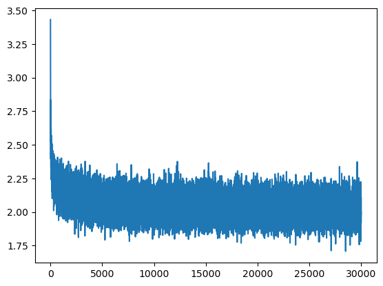
The loss curve decreases overall but exhibits some variance, indicating that further hyperparameter tuning could improve performance. The initial ‘hockey-stick’ shape might also be mitigated with a better weight initialization strategy. However, for our purposes, we can proceed with the current setup and keep the approach simple.

Evaluation (Held-out Mini-batch)

Evaluation is done on unseen data. We disable gradient tracking with torch.no_grad, switch to evaluation mode, and compute both loss and accuracy.

@torch.no_grad()
def eval_minibatch():
    model.eval()
    idx    = torch.randint(0, Xtst.size(0), (4096,), device=device)
    logits = model(Xtst[idx])                 # (B, V)
    y      = Ytst[idx]                        # (B,)
    loss   = F.cross_entropy(logits, y).item()
    acc    = (logits.argmax(1) == y).float().mean().item()  # [docs](https://pytorch.org/docs/stable/generated/torch.argmax.html)
    model.train()
    return loss, acc

val_loss, val_acc = eval_minibatch()
print(f"val loss: {val_loss:.4f} | val acc: {val_acc:.3f}")

With this setup, the model is no longer just a table of counts. It is a trainable system that builds its own internal representations. Even with a fixed 3-character window, we can already see the core ingredients of modern language models at work: embeddings, nonlinear layers, and iterative optimization.

8. Sampling & Decoding

Training gives us losses and accuracies, but sampling turns those numbers into names. Generation is just sampling: repeatedly draw the next token from the model’s conditional distribution until EOS is reached.

@torch.no_grad()
def generate(n_samples=10, maxlen=15):
    model.eval()
    V = len(itos)

    for _ in range(n_samples):
  
        ctx = torch.zeros((1, block_size), dtype=torch.long, device=device)  
        s = []

        for _ in range(maxlen):
            logits = model(ctx)                          # (1, V) logits

            # convert logits into probabilities
            probs = F.softmax(logits, dim=1)             # (1, V) [docs](https://pytorch.org/docs/stable/generated/torch.nn.functional.softmax.html)

            # sample from the distribution
            next_idx = torch.multinomial(probs, 1)       # (1, 1)
            ix = next_idx.item()

            ch = itos[ix]
            if ch == "?":
                break
            s.append(ch)

            # slide the window forward
            ctx = torch.roll(ctx, shifts=-1, dims=1)     # still (1, block_size) [docs](https://pytorch.org/docs/stable/generated/torch.roll.html)
            ctx[0, -1] = ix

        print("".join(s))

Generation proceeds by starting with SOS tokens, repeatedly sampling from the softmax distribution, and shifting the context forward until EOS or max length is reached.

Example Outputs:

askiem
alerindro
richardin
fulayma
marian
jhona
nodou
chris
saurie
nardi
enni
giadan
serena
bessa
emma

Some outputs (marian, serena, emma) are plausible Italian names; others (askiem, fulayma) are hybrids that never appeared in training. This balance is exactly what we expect: the model has internalized local character regularities but lacks the longer memory needed for fully natural names. Sampling exposes both strengths and limits: the model generalizes beyond memorization but still lacks long-range structure.

9. Analysis

With both the count-based bigram model and the neural 3-gram model trained, we can now compare them quantitatively.

Quantitative Comparison

On the held-out test set:

# Bigram test loss
with torch.no_grad():
    log_probs = torch.log(probs[Xtst, Ytst])
    loss_bigram = -log_probs.mean().item()

# Neural 3-gram test loss 
val_loss = F.cross_entropy(model(Xtst), Ytst).item()
print(loss_bigram, val_loss)

Results:

• Bigram loss ≈ 2.48
• Neural 3-gram loss ≈ 2.09

The reduction of ~0.4 bits per character means the trigram model assigns systematically sharper probabilities, leading to fewer mistakes across the sequence. Even small cross-entropy reductions compound over long sequences.

The Role of Context

• Bigram: memory of one token → captures only immediate adjacency.
• Neural 3-gram: memory of three tokens → smoother, more realistic local patterns.
• General rule: longer contexts reduce uncertainty by conditioning on more history, but they demand architectures (and data/compute) that can handle the growth in parameters and estimation complexity.

In short, language modeling is a trade-off between expressiveness (how much structure longer context can capture) and feasibility (how much compute and data are required). Modern models (RNNs → Transformers) push this frontier by scaling effective context to entire sequences.

10. Conclusion

We set out to generate plausible Italian names via next-character prediction. From count-based bigrams to a neural trigram, we made the math explicit (MLE, softmax, cross-entropy) and showed how fixed counts become learnable functions through embeddings and nonlinear layers.

Key Lessons

At heart, a language model factorizes

with effectiveness governed by how much context it conditions on. (Chain rule)

• Neural models generalize counts. With one-hot inputs, an embedding + MLP can reproduce the bigram table; added capacity captures patterns not observed verbatim.
• Empirical signal matters. Test cross-entropy dropped from ~2.48 to ~2.09 nats, indicating systematically sharper predictions.
• Context length limits performance. More history improves coherence but requires more data and compute.

Big Picture

Language modeling has always fought with context. Classical n-grams blow up combinatorially, while small neural nets manage only modest extensions. Modern models—RNNs and especially Transformers—address this by reusing and sharing parameters, scaling context from a handful of characters to entire documents.

Next up: attention—the mechanism that lets models capture dependencies across any distance without the n-gram blow-up. In the following post we’ll unpack Attention Is All You Need and see how it unlocks the long-range structure behind today’s transformers.