Neural Network Training: Statistics, Initialization and Diagnostics

Introduction

This post comes from a cleaned-up version of the notes I wrote while studying neural network training. The goal is to turn those notes into something more readable, without losing the practical and exploratory style of the original work.

In these notes I dive into a set of concepts that are fundamental for understanding how neural networks work and why they behave in a certain manner during training. These ideas are not only useful for building intuition, but also essential for debugging models, diagnosing training instabilities, and making optimization behave properly.

The topics covered are:

• basic statistical concepts and useful probability distributions
• model outputs, softmax, and what to expect from the initial loss
• backpropagation
• common problems that arise during training
• how initialization affects training, how variance propagates across layers, and some signal-processing intuition behind these effects
• diagnostic tools and training KPIs
• architectural mechanisms that patch these problems

The code and plots in this post are developed from a notebook, available in this GitHub repository: Neural-Network-Statistic-and-diagnostic-tools.

Statistics & Distributions

Firstly we have to introduce some basic concepts, starting from the definition of a random variable.

We define $X$ as a random variable when $X$ represents the possible outcomes of a random process. This allows us to model uncertainty mathematically and to reason about events such as the probability that $X$ falls inside a certain range.

Random variables fall into two main categories:

• Discrete random variables
• Continuous random variables

The main difference lies in the values that $X$ can assume. A discrete random variable can assume values from a finite or countable set, while a continuous random variable can assume infinitely many values inside an interval.

Every distribution is characterized by functions that describe how probability is assigned. For continuous random variables, the most important one is the probability density function, or pdf.

The pdf can be misleading at first, because it does not directly give the probability that $X$ is equal to a specific value. Instead, it describes density. Probabilities are obtained by integrating the density over an interval:

This also means that the probability of a single exact value is zero:

So the intuitive interpretation is that probability is the area under the pdf curve.

The cumulative distribution function, or cdf, accumulates this area from $-\infty$ up to a value $x$:

Usually in machine learning we are interested in continuous random variables, and one of the most important examples is the Gaussian distribution.

For a Gaussian random variable $X \sim \mathcal{N}(\mu, \sigma^2)$, the probability density function is:

In this case, the probability that $X$ falls between $a$ and $b$ is:

The parameters $\mu$ and $\sigma^2$ are respectively the mean and the variance of the distribution. The mean describes where the distribution is centered, while the variance describes how spread out the values are around the mean.

Their theoretical definitions are:

When we work with data, we usually do not know the true distribution parameters. We only have samples, so we estimate the mean and variance from them.

Given samples $x_1, x_2, \dots, x_n$, the sample mean is:

The sample variance is:

So basically the mean is derived from averaging the values, and the variance is derived by seeing how each value differs from the mean. We square these differences, average them, and obtain a measure of how spread out the samples are around the mean. If you have noticed that in the second case we do not average by $n$ but by $n - 1$, I suggest you read this explanation.

Now that we have defined these basic concepts, we can use Python and PyTorch to build some intuition through examples. We can use these tools to generate samples from a standard Gaussian distribution:

plt.figure(figsize=(12, 8))
bins = torch.linspace(-4, 4, 51).numpy()

for idx, i in enumerate((100, 1000, 10000, 100000), start=1):
    x = torch.randn(i)
    mean = x.mean()
    variance = x.var(unbiased=True)

    plt.subplot(2, 2, idx)
    plt.hist(x.numpy(), bins=bins, density=True, alpha=0.7, color="g")
    plt.title(f"n = {i}\nmean = {mean:.3f}, var = {variance:.3f}")

plt.tight_layout()
plt.show()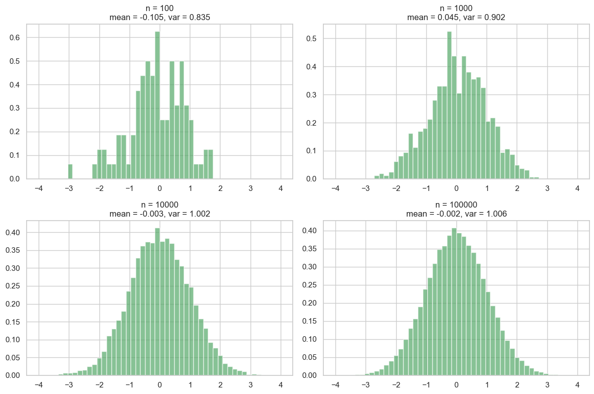

As we can see, with a small number of samples, the mean and variance can deviate significantly from their true values (0 and 1 for a standard normal distribution). As we increase the number of samples, the estimates become more accurate, and the histogram approaches the shape of the true Gaussian distribution. If you are interested to delve deeper, this is related to the law of large numbers and the central limit theorem.

Now we can see intuitively how mean and variance modify the shape of the bell curve, that is, the plot of the Gaussian distribution over a histogram. The mean shifts the center of the bell curve, while the variance controls how wide or narrow it is. A higher variance results in a wider bell curve, while a lower variance results in a narrower bell curve.

plt.figure(figsize=(12, 10))
bins = torch.linspace(-8, 8, 80).numpy()

plt.subplot(2, 1, 1)
for mu in (-3, 0, 3):
    x = torch.randn(10000) + mu
    plt.hist(x.numpy(), bins=bins, density=True, alpha=0.5, label=f"mu = {mu}")

plt.title("Fixed variance, changing mean")
plt.legend()

plt.subplot(2, 1, 2)
for sigma in (0.5, 1, 2):
    x = torch.randn(10000) * sigma
    plt.hist(x.numpy(), bins=bins, density=True, alpha=0.5, label=f"sigma = {sigma}")

plt.title("Fixed mean, changing variance")
plt.legend()

plt.tight_layout()
plt.show()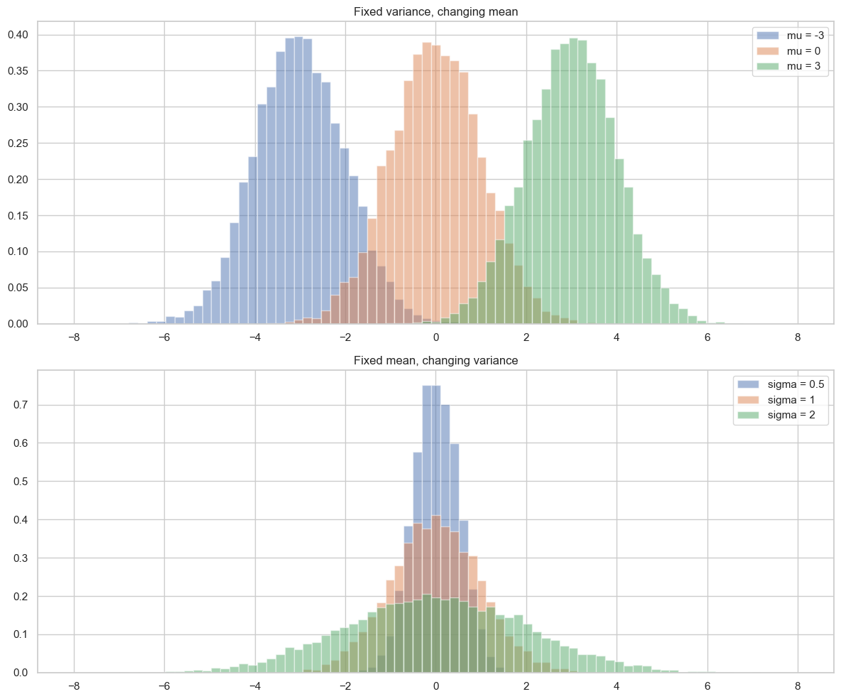

Now that we have built some intuition about these concepts, we can look at what happens when we apply a nonlinear transformation to samples drawn from a random variable. In our context, we want to see how an initially Gaussian distribution changes when we apply the tanh activation function.

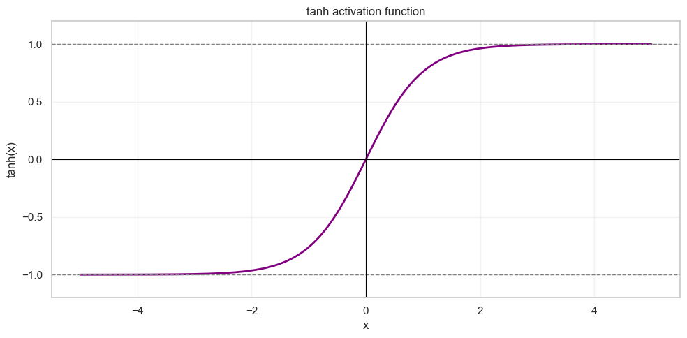
The tanh activation function is defined as follows:

Its output is bounded between $-1$ and $1$:

If we apply tanh to every sample and then plot the result, we can see that the output distribution is no longer Gaussian. Its mean and variance are changed by the nonlinearity:

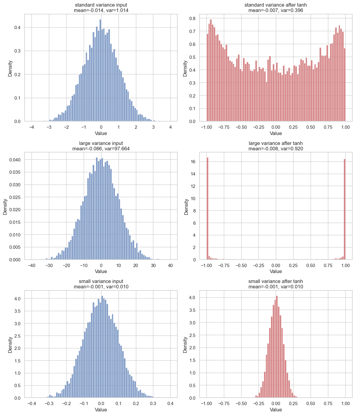
The most important thing to grasp is that the output distribution depends strongly on the input variance. When the variance is large, many input values fall far from the mean. Since tanh is almost flat for large positive or negative values, those samples are pushed close to $-1$ or $1$. This is called tanh saturation, and we will come back to it later.

On the other hand, when the variance is small, most values stay close to $0$. Around zero, tanh is almost linear, so the transformed values also remain close to zero. You can see it respectively in row 2 and row 3 of the image.

Neural Network Model

To follow along during the explanation we are going to use a simple neural network from the previos post. The context is the same, we have a datasets composed of names and we are trying to train a bigram model to learn how to generate italian names.

# MLP 
n_embd = 10 # the dimensionality of the character embedding vectors
n_hidden = 200 # the number of neurons in the hidden layer of the MLP

g = torch.Generator().manual_seed(2147483647) # for reproducibility
C  = torch.randn((vocab_size, n_embd),            generator=g)
W1 = torch.randn((n_embd * block_size, n_hidden), generator=g)#* ((5/3)/(n_embd*block_size)**0.5)
b1 = torch.randn(n_hidden,                        generator=g)#*0.01
W2 = torch.randn((n_hidden, vocab_size),          generator=g)*0.01
b2 = torch.randn(vocab_size,                      generator=g)*0


parameters = [C, W1, b1, W2, b2]
print(sum(list((p.nelement() for p in parameters)))) # number of parameters in total
for p in parameters:
    p.requires_grad = True

# same optimization as last time
max_steps = 200000
batch_size = 32
lossi = []

for i in range(max_steps):
  
  # minibatch construct
  ix = torch.randint(0, Xtr.shape[0], (batch_size,), generator=g)
  Xb, Yb = Xtr[ix], Ytr[ix] # batch X,Y
  
  # forward pass
  emb = C[Xb] # embed the characters into vectors
  embcat = emb.view(emb.shape[0], -1) # concatenate the vectors
  hpreact = embcat @ W1 #+ b1 # hidden layer pre-activation

  h = torch.tanh(hpreact) # hidden layer
  logits = h @ W2 + b2 # output layer
  loss = F.cross_entropy(logits, Yb) # loss function
  
  # backward pass
  for p in parameters:
    p.grad = None
  loss.backward()
  
  # update
  lr = 0.1 if i < 100000 else 0.01 # step learning rate decay
  for p in parameters:
    if p.grad is not None:
      p.data += -lr * p.grad
  
  # track stats
  if i % 10000 == 0: # print every once in a while
    print(f'{i:7d}/{max_steps:7d}: {loss.item():.4f}')
  lossi.append(loss.log10().item())

As you can see the model and the forward pass are pretty simple, we have the following:

• ix: random indices used to sample a minibatch from the training set. Shape: (batch_size,).
• Xb: input batch, obtained with Xtr[ix]. Each row contains the context characters used to predict the next one. Shape: (batch_size, block_size).
• Yb: target batch, obtained with Ytr[ix]. Each element is the correct next character index. Shape: (batch_size,).
• emb = C[Xb]: embedding lookup. Each character index in Xb is replaced by its learned vector from C. Shape: (batch_size, block_size, n_embd).
• embcat = emb.view(emb.shape[0], -1): concatenation of the context embeddings into a single vector per example. Shape: (batch_size, block_size * n_embd).
• hpreact = embcat @ W1: hidden layer pre-activation, before applying the nonlinearity. Shape: (batch_size, n_hidden).
• h = torch.tanh(hpreact): hidden layer activation. Shape: (batch_size, n_hidden).
• logits = h @ W2 + b2: raw output scores, one score for each possible next character. Shape: (batch_size, vocab_size).
• loss = F.cross_entropy(logits, Yb): compares the logits with the correct targets and returns a scalar loss. Shape: ().

Cross-Entropy Loss and Output Scale

At the end of the network we obtain logits, one raw score for each possible next character. These are not probabilities yet. They can be any real number, positive or negative.

In PyTorch, F.cross_entropy(logits, Yb) expects these raw logits directly.

Under the hood, PyTorch's cross-entropy combines two operations:

log_probs = F.log_softmax(logits, dim=1)
loss = F.nll_loss(log_probs, Yb)

So when we write:

loss = F.cross_entropy(logits, Yb)

we are already doing the stable version of softmax + negative log-likelihood.

For a single example, let:

be the logits, where $V$ is the vocabulary size. Softmax turns these raw scores into probabilities:

This does two things: it makes every value positive, and it normalizes all values so that they sum to one:

So after softmax we can interpret $p_i$ as the probability assigned to token $i$.

Log-softmax does the same transformation, but directly in log space:

This is the numerically stable quantity used by the loss. If the correct target class is $y$, the negative log-likelihood is:

So the loss is small when the model assigns high probability to the correct token, and large when it assigns low probability to it.

Softmax is still useful as intuition. If the logits are close to each other, the output distribution is close to uniform. If one logit is much larger than the others, softmax puts most of the mass on that class.

So the scale of the final logits matters. Small logits usually mean a softer, less confident output distribution. Very large logits usually mean a very sharp, overconfident distribution.

g_softmax = torch.Generator().manual_seed(2147483647)

for scale in (0.1, 1.0, 10.0):
    logits = torch.randn(4, generator=g_softmax) * scale
    probs = torch.softmax(logits, dim=0)

    print(f"scale = {scale}")
    print("logits:", logits.round(decimals=3))
    print("probs :", probs.round(decimals=3))
    print()

scale = 0.1
logits: tensor([-0.0980, -0.1660, -0.0060, -0.0340])
probs : tensor([0.2440, 0.2280, 0.2680, 0.2600])

scale = 1.0
logits: tensor([ 2.0990,  0.8960,  0.3380, -0.2090])
probs : tensor([0.6360, 0.1910, 0.1090, 0.0630])

scale = 10.0
logits: tensor([ -9.3910, -11.8100,  -6.2840,  -9.8260])
probs : tensor([0.0420, 0.0040, 0.9280, 0.0270])

This is why the magnitude of the final layer matters at initialization. At the beginning of training, the model has not learned anything yet, so it should not be very confident about any particular token. Its predictions should be close to uniform, and the loss should start near the baseline log(vocab_size):

expected_initial_loss = torch.tensor(vocab_size).float().log()
print("vocab_size:", vocab_size)
print("expected initial loss:", expected_initial_loss.item())

vocab_size: 27
expected initial loss: 3.295836925506592

If the actual initial loss is much higher than this value, something is wrong with the initialization. The model is not just random: it is confidently random. It assigns too much probability to wrong classes, and cross-entropy punishes that heavily.

This is exactly what creates the initial hockey-stick shape in the training loss curve:

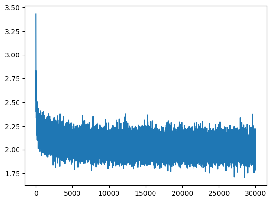
The loss starts too high, then quickly drops once the model learns to reduce its overconfident random predictions. But this early drop is not meaningful learning: it is mostly the model correcting a bad output scale.

A simple fix is to initialize the last layer with smaller weights:

W2 = torch.randn((n_hidden, vocab_size), generator=g) * 0.01
b2 = torch.randn(vocab_size, generator=g) * 0

We can see the effect directly by comparing a large output-layer scale with a smaller one:

g_compare = torch.Generator().manual_seed(2147483647)
batch_size = 32
ix = torch.randint(0, Xtr.shape[0], (batch_size,), generator=g_compare)
Xb, Yb = Xtr[ix], Ytr[ix]

C_test = torch.randn((vocab_size, n_embd), generator=g_compare)
W1_test = torch.randn((n_embd * block_size, n_hidden), generator=g_compare) * ((5/3) / (n_embd * block_size)**0.5)

emb = C_test[Xb]
embcat = emb.view(emb.shape[0], -1)
hpreact = embcat @ W1_test
h = torch.tanh(hpreact)

for scale in (1.0, 0.01):
    W2_test = torch.randn((n_hidden, vocab_size), generator=g_compare) * scale
    b2_test = torch.zeros(vocab_size)
    logits = h @ W2_test + b2_test
    loss = F.cross_entropy(logits, Yb)

    print(f"W2 scale = {scale}")
    print("logits std:", logits.std().item())
    print("loss:", loss.item())
    print()

W2 scale = 1.0
logits std: 10.497655868530273
loss: 25.23309326171875

W2 scale = 0.01
logits std: 0.11374638229608536
loss: 3.3066704273223877

This keeps the initial logits close to zero. When logits are close to zero, softmax would produce probabilities close to uniform, and the initial loss starts near the theoretical baseline.

Now we can train again with this initialization and plot the loss curve. To make the trend easier to read, we average the loss every 1000 iterations:

# Now we can plot the loss curve to see how it evolves during training
plt.figure(figsize=(10, 5))
lossi_avg = torch.tensor(lossi).view(-1, 1000).mean(1)
plt.plot(lossi_avg, label="Training Loss (log10)")
plt.axvline(100, color="r", linestyle="--", label="learning-rate decay")
plt.xlabel("1000-iteration blocks")
plt.ylabel("log10(loss)")
plt.legend()
plt.show()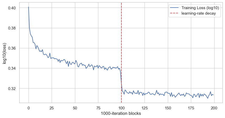

Each point is the average of 1000 consecutive training iterations. The vertical line is at block 100, which corresponds to iteration 100000, where the learning rate changes from 0.1 to 0.01. With the smaller last-layer initialization, the curve no longer starts with the same artificial hockey-stick drop.

Manual BackPropagation through the net

Now we want to understand what happens under the hood when we call:

loss.backward()

The loss is just a function of all the parameters of the network:

Training means changing these parameters in the direction that reduces the loss. For each parameter $\theta$, PyTorch computes:

This tells us how much the loss changes when that parameter changes a little.

Then the update step is:

where $\eta$ is the learning rate.

In code, this is the part:

# backward pass
for p in parameters:
    p.grad = None
loss.backward()

# update
lr = 0.1 if i < 100000 else 0.01 # step learning rate decay
for p in parameters:
    if p.grad is not None:
        p.data += -lr * p.grad

First we reset the old gradients, then .backward() computes the new gradients, and finally we move every parameter in the opposite direction of its gradient.

The key mathematical tool is the chain rule. If a function is built by composing smaller functions:

then:

Backpropagation is just repeated chain rule applied from the loss backward through the network.

To make the mechanism clear, we do not start from the full neural network. We start from a single simplified block:

So the full computation is a composition of functions:

During the forward pass we go from left to right. During backpropagation we go from right to left.

The first gradient comes from the loss itself:

Since:

we have:

This depends on the specific loss function. In the previous section we used cross-entropy. For softmax + cross-entropy, the gradient with respect to the logits has the clean form:

Here, in the simplified example, we just call the first gradient:

Now we move one step backward. Since:

we want to know how the loss changes when $z$ changes. This is a two-function composition:

So the chain rule gives:

The local derivative of tanh is:

Since $y = \tanh(z)$, this is also:

Therefore:

This quantity is the gradient that arrives at the linear part.

Now we move one more step backward. The linear part is:

There are three things we may care about: $w$, $b$, and $x$.

First, for the weight $w$:

so:

Since:

we get:

For the bias $b$:

so:

Since:

we get:

For the input $x$:

so:

Since:

we get:

So the full backward pass for this small block is:

This is the core idea. Each operation receives a gradient from the operation after it, multiplies it by its own local derivative, and passes the result backward.

The full neural network is just the same mechanism repeated many times, with vectors and matrices instead of single numbers.

Nonlinearities, tanh saturation, and local gradient attenuation

Now that we have seen what happens to a Gaussian distribution when it is passed through a tanh, and now that we know the local derivative of tanh, we can connect the two ideas.

The question is: what kind of distribution does a neuron see before the nonlinearity?

Consider one neuron:

or, more compactly:

This value $z$ is the pre-activation. It is the input of the tanh:

To understand the scale of $z$, we need two basic facts about variance.

First, if random variables are independent, the variance of their sum is the sum of their variances:

Second, multiplying a random variable by a constant scales the variance by the square of that constant:

In our neuron, each term is $w_i x_i$. If we assume that the inputs and weights are independent and centered around zero, then the variance of the pre-activation is approximately:

and, under the usual independence assumptions:

From now on, assume that the input activations are normalized so that:

Then the expression becomes:

This is the key point: under this assumption, the variance of the pre-activation grows with the number of inputs, also called fan_in.

If the weights are initialized too large, then $\mathrm{Var}(w)$ is large, so $\mathrm{Var}(z)$ becomes large. This means that many pre-activations fall far from zero.

But we already saw what tanh does in that case: it pushes large positive values close to $1$ and large negative values close to $-1$.

So if $z$ has high variance, then:

will be concentrated near $-1$ and $1$.

This is a problem for backpropagation because the local derivative of tanh is:

If $h \approx 1$ or $h \approx -1$, then:

So the gradient that flows backward through the tanh gets multiplied by a number close to zero:

This is local gradient attenuation. If many neurons are saturated, many gradients are killed locally. This is one way vanishing gradients appear in practice.

We can see this directly in the network by plotting the hidden activations. Here we are still using the naive hidden-layer initialization: W1 is not fan-in normalized yet, while W2 is already scaled down to fix the initial output confidence.

plt.hist(h.view(-1).tolist(), 50);

If a large amount of mass is close to -1 and 1, the hidden layer is saturated.

An even clearer diagnostic is:

plt.figure(figsize=(10, 20))
plt.imshow(h.abs() > 0.99, cmap="grey", interpolation="nearest");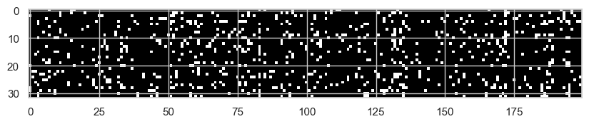

Each white point is an activation with absolute value greater than 0.99. These are neurons that are almost fully saturated. For those values, the local tanh derivative is almost zero, so the gradient does not flow well through them.

The opposite problem is when the weights are initialized too small.

If $\mathrm{Var}(w)$ is too small, then:

also becomes too small. In this case most pre-activations are very close to zero.

For tanh, this does not kill the local gradient, because around zero:

and:

So the tanh itself is not saturated. The problem is more subtle: the activations are small because the pre-activations are small.

If the next layer is:

then the gradient of the loss with respect to the next weight matrix has the usual form:

where $\delta_{next}$ is the gradient arriving from the next pre-activation. So if $h$ is very small, the weight gradient is also small. The update becomes small not because tanh blocked the gradient locally, but because the activation that multiplies the gradient is tiny.

There is a second effect in the backward pass. The gradient sent to the previous layer is:

If the weights are very small, this backward signal is also scaled down. So with weights that are too small, the network can end up with small activations in the forward pass and small gradients in the backward pass.

So we want a middle ground:

• not too large, otherwise tanh saturates and gradients vanish;
• not too small, otherwise the signal becomes tiny;
• roughly stable variance from layer to layer.

It is important to be precise about what we are analyzing here. This is an initialization problem. We are looking at what happens at the first forward pass, before training has had the chance to move the parameters.

Later, during training, similar problems can appear again: activations can drift, distributions can shift, and neurons can still move into saturated regions. That is a different problem, and later we will look at mechanisms designed to keep activations well behaved during training.

For now, we only want a good starting point.

From:

and assuming:

we get:

So if we want:

we need:

which means:

and therefore:

This gives us a very simple first correction: scale the weights by the inverse square root of the fan-in.

W1 = torch.randn((n_embd * block_size, n_hidden), generator=g) * (1 / (n_embd * block_size)**0.5)

This does not solve every training problem, but it fixes the first obvious one: the pre-activations are no longer exploding just because each neuron is summing many independent inputs.

After this change, we can rerun the same saturation diagnostic:

plt.figure(figsize=(10, 20))
plt.imshow(h.abs() > 0.99, cmap="grey", interpolation="nearest");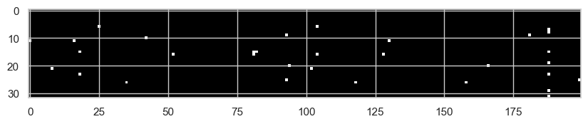

We can also look again at the activation histogram:

plt.hist(h.view(-1).tolist(), 50);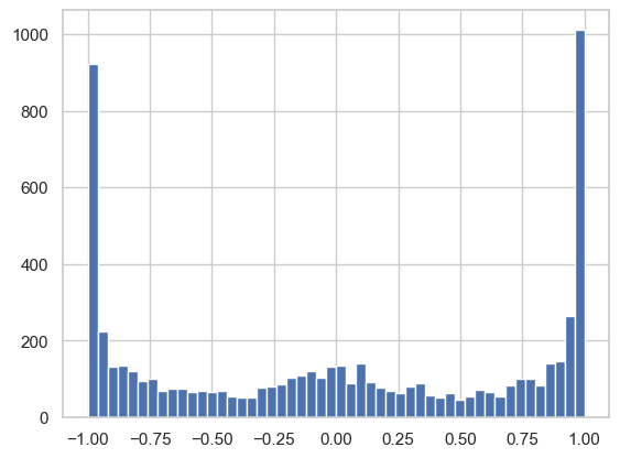

Now we see far fewer saturated activations, because the initial pre-activation variance has been brought back to a reasonable scale. Clearly, there are more advanced techniques to adjust weights at initialization, such as Xavier/Glorot initialization, He/Kaiming initialization, and Fixup initialization.

But later we are going to see that we can introduce some architectural changes that helps us take in control both the initialization and in training variance problem.

Modern stabilization mechanisms

In this section we are going to see some of the most common techniques used in modern neural networks to keep activations and gradients well behaved during training. These techniques are not just for initialization: they help maintain stable distributions throughout training, which is crucial for deep networks.

Batch Normalization

Batch Normalization was introduced by Sergey Ioffe and Christian Szegedy in the Google paper Batch Normalization: Accelerating Deep Network Training by Reducing Internal Covariate Shift.

Until now we mostly reasoned about initialization. We asked: if the input variance is approximately one, how should we initialize the weights so that the pre-activation variance does not explode or collapse at the first forward pass?

That is important, but it is only the first forward pass.

During training, the weights of the previous layers keep changing. So the distribution seen by a layer also keeps changing. A layer may start with reasonable pre-activations, but after some updates those pre-activations can shift, widen, shrink, or move into the saturated region of the nonlinearity. This is the idea that the BatchNorm paper calls internal covariate shift: the input distribution of internal layers is not stable while the model is training.

The idea of BatchNorm is simple:

before sending the pre-activations into the nonlinearity, normalize them over the mini-batch.

In our case, the block becomes:

So the tanh does not directly see the raw linear output anymore. It sees a normalized version of it.

To understand the mechanism, start from the usual standardization formula. If:

then:

has:

and:

If the original variable is Gaussian, then this produces a standard Gaussian:

BatchNorm applies exactly this idea inside the network, but using mini-batch statistics instead of the true population mean and variance.

Suppose the linear layer output has shape:

where m is the batch size and d is the number of neurons. Each column of z is one neuron evaluated over all examples in the batch. So BatchNorm normalizes each neuron independently across the batch.

For one neuron, we have the mini-batch values:

The batch mean is:

The batch variance is:

Then we normalize:

The small $\epsilon$ is only for numerical stability, so we never divide by zero.

At this point, for each neuron, the batch of normalized values has approximately zero mean and unit variance. This does not magically make every distribution Gaussian, but if the pre-activation is already roughly Gaussian, it brings it close to a standard Gaussian.

There is one more important detail. If we forced every layer to always use zero-mean and unit-variance activations, we would reduce what the network can represent. Sometimes the network may actually want a shifted or scaled version of the normalized activation.

So BatchNorm adds two learnable parameters per neuron:

where:

• $\gamma$ is a learnable scale
• $\beta$ is a learnable shift

This is crucial. BatchNorm normalizes the signal, but then gives the model the freedom to learn the right scale and offset again if that is useful.

This is the implementation used in the notebook:

class BatchNormalizationLayer:
    def __init__(self, fan_out, eps=1e-5, momentum=0.1):
        self.eps = eps
        self.momentum = momentum
        self.training = True

        self.gamma = torch.ones(fan_out, requires_grad=True)
        self.beta = torch.zeros(fan_out, requires_grad=True)

        self.running_mean = torch.zeros(fan_out)
        self.running_var = torch.ones(fan_out)

    def __call__(self, x):
        if self.training:
            batch_mean = x.mean(0)
            batch_var = x.var(0, unbiased=False)

            x_normalized = (x - batch_mean) / torch.sqrt(batch_var + self.eps)

            with torch.no_grad():
                self.running_mean = (1 - self.momentum) * self.running_mean + self.momentum * batch_mean
                self.running_var = (1 - self.momentum) * self.running_var + self.momentum * batch_var
        else:
            x_normalized = (x - self.running_mean) / torch.sqrt(self.running_var + self.eps)

        out = self.gamma * x_normalized + self.beta
        self.out = out
        return out

    def parameters(self):
        return [self.gamma, self.beta]

The important line is:

batch_mean = x.mean(0)
batch_var = x.var(0, unbiased=False)

The dimension 0 is the batch dimension. So we are not computing one global mean over the whole matrix. We are computing one mean and one variance for each neuron.

Then:

x_normalized = (x - batch_mean) / torch.sqrt(batch_var + self.eps)

standardizes every column independently.

The parameters:

self.gamma = torch.ones(fan_out, requires_grad=True)
self.beta = torch.zeros(fan_out, requires_grad=True)

are the learnable scale and shift. They are returned by parameters(), so the optimizer updates them like normal weights.

The running statistics are needed because training and inference are different. During training, using the current mini-batch statistics is fine. During inference, instead, we do not want the prediction for one example to depend on the other examples that happened to be in the same batch. So we use the running estimates accumulated during training:

self.running_mean = (1 - self.momentum) * self.running_mean + self.momentum * batch_mean
self.running_var = (1 - self.momentum) * self.running_var + self.momentum * batch_var

In the model, we insert BatchNorm after the linear layer and before the tanh:

layers = [
   Linear(n_embd * block_size, n_hidden),
   BatchNormalizationLayer(n_hidden),
   Tanh(),
   Linear(n_hidden, n_hidden),
   BatchNormalizationLayer(n_hidden),
   Tanh(),
   Linear(n_hidden, vocab_size),
]

This placement matters. The paper also discusses applying BatchNorm before the nonlinearity, because the goal is to keep the nonlinearity input in a controlled range. For us this means: normalize the pre-activation, then apply tanh.

There is also a small practical consequence: if we normalize the output of xW + b, the bias before BatchNorm becomes less important, because subtracting the batch mean removes constant shifts. The learnable $\beta$ after normalization becomes the meaningful shift.

We will inspect the concrete effect in the diagnostics section below. The important point here is conceptual: initialization tries to make the first step healthy; BatchNorm keeps re-normalizing the signal while the network is changing.

Layer Normalization

Layer Normalization was introduced by Ba, Kiros and Hinton in Layer Normalization.

The idea is close to BatchNorm, but the axis is different.

BatchNorm normalizes each neuron using the statistics of the mini-batch. So it looks across examples:

LayerNorm, instead, normalizes the channel vector of a single example.

This is the version that will be very useful when we move to transformers. In a transformer, each token is represented by a vector:

where $t$ is the token position and $d$ is the number of channels, or embedding dimensions.

LayerNorm takes this vector and normalizes it across its channels:

and then, as usual, it gives the model a learnable scale and shift:

The important intuition is this: for each token, LayerNorm asks "is this token vector well scaled across its channels?" It does not need to look at the other examples in the batch.

That is why it fits transformers so naturally. When we predict the next token, every token representation is a channel vector that is repeatedly processed by attention and MLP blocks. LayerNorm keeps those token vectors in a reasonable scale before or after the block, depending on the architecture.

So for now I only want to remember the operational difference:

• BatchNorm normalizes using the batch dimension
• LayerNorm normalizes using the channel dimension of each single token/example

Residual connections

Another modern mechanism that directly attacks the training problem is the residual connection, introduced by He, Zhang, Ren and Sun in Deep Residual Learning for Image Recognition.

The problem is very pragmatic. We would like to make networks deeper, because deeper networks should be able to build more abstract representations. But after some point, simply stacking more layers does not automatically help. The optimization becomes harder, gradients have to pass through many transformations, and the deeper model can even train worse than a shallower one.

The residual idea is to stop forcing a block to learn the whole transformation from scratch.

Without a residual connection, a block learns:

With a residual connection, the block learns:

This changes the meaning of what the block has to learn. The block is not asked to produce the full output anymore. It only has to learn a correction to the input.

That is why the name is residual: $F(x)$ is the residual part, the difference between what we already have and what we want.

If the best thing for a layer is to do almost nothing, the residual block can learn:

and then:

So the block can behave like an identity mapping. This is important because adding more layers should not make the optimization problem worse just because the model has to rediscover how to copy information forward.

There is also a direct gradient intuition. If:

then:

So during backpropagation the gradient has a direct path through the identity term. It does not have to pass only through the nonlinear block $F$. This does not mean gradients can never vanish or explode, but it gives the network a much cleaner route for information and gradients to flow through depth.

In code, the idea is basically:

x = x + block(x)

or, if the dimensions need to be adapted:

x = projection(x) + block(x)

This is why residual connections fit naturally in this discussion. BatchNorm tries to keep the internal distributions under control. Good initialization tries to make the first forward/backward pass reasonable. Residual connections make depth easier by giving the network a stable path that can carry both activations and gradients across many layers.

Dropout

Dropout was introduced by Srivastava, Hinton, Krizhevsky, Sutskever and Salakhutdinov in Dropout: A Simple Way to Prevent Neural Networks from Overfitting.

The motivation is different from BatchNorm and residual connections.

BatchNorm and residual connections mainly help with optimization and signal flow. Dropout is mostly a regularization technique: it tries to prevent the network from fitting the training data too specifically.

The idea is simple. During training, for each neuron we sample a Bernoulli random variable that decides if that neuron is active or not.

where $p$ is the probability that the neuron is kept active.

If the sampled value is 1, the neuron fires and its activation is used. If the sampled value is 0, the neuron is switched off for that forward pass.

So at every training step, the network is slightly different. Some neurons are present, some neurons do not fire. The model cannot rely too much on one specific activation always being there.

The intuition is that dropout forces redundancy. If a feature is useful, the network should not encode it in one fragile path only. It should learn representations that still work even when some neurons are temporarily off.

Dropout is not something I would add blindly to fix a broken training run. If activations are saturated or gradients are dead, dropout does not solve that. It can even make optimization noisier. But once the model trains and starts to overfit, dropout is a clean way to make the network less dependent on exact neuron co-adaptations.

So in the mental map:

• initialization controls the first signal scale
• BatchNorm controls internal statistics during training
• residual connections help activations and gradients travel through depth
• dropout regularizes the representation by making it robust to missing units

Diagnostics and training KPIs

At this point, only looking at the loss is not enough.

The loss tells us if the model is improving, but it does not tell us why the training is healthy or unhealthy. If the loss is bad, the problem could be saturated activations, gradients that are too small, gradients that are too large, or updates that are completely out of scale with the parameters.

So we need a small diagnostic toolbox.

Loss curve

The first plot is still the loss curve. But we do not plot every single iteration, because that is too noisy. We average every 1000 iterations:

# Now we can plot the loss curve to see how it evolves during training
plt.figure(figsize=(10, 5))
lossi_avg = torch.tensor(lossi).view(-1, 1000).mean(1)
plt.plot(lossi_avg, label="Training Loss (log10)")
plt.axvline(100, color="r", linestyle="--", label="learning-rate decay")
plt.xlabel("1000-iteration blocks")
plt.ylabel("log10(loss)")
plt.legend()
plt.show()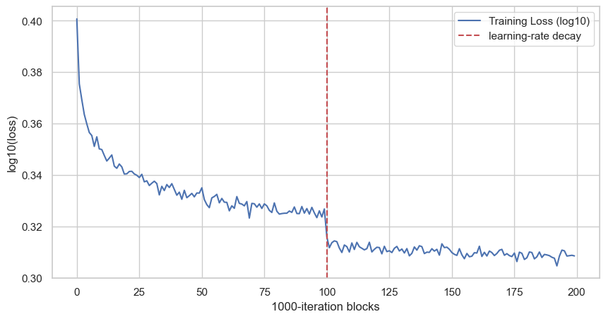

This gives us the global view. The model improves quickly at the beginning, then the curve becomes flatter. The red dashed line is the learning-rate decay: after 100 blocks, so after 100000 iterations, the learning rate goes from 0.1 to 0.01.

This plot is useful, but it is not enough. It tells us that training is moving, but it does not tell us what is happening inside the network.

Saturated activations

Since we are using tanh, the first thing I want to inspect is saturation. A tanh neuron is saturated when its output is very close to -1 or 1. In that region, the local derivative is close to zero, so the gradient has a hard time flowing backward.

The following plot shows, for each Tanh layer, which activations are saturated:

# Visualize saturated activations for the two Tanh layers
tanh_layers = [(i, layer) for i, layer in enumerate(layers[:-1]) if isinstance(layer, Tanh)]

plt.figure(figsize=(10, 4 * len(tanh_layers)))

for k, (i, layer) in enumerate(tanh_layers, 1):
    t = layer.out.detach()

    plt.subplot(len(tanh_layers), 1, k)
    plt.imshow((t.abs() > 0.99).float(), cmap="gray", interpolation="nearest", aspect="auto")
    plt.title(f'layer {i} ({layer.__class__.__name__}) | saturated activations')
    plt.xlabel('neuron index')
    plt.ylabel('batch example')

plt.tight_layout()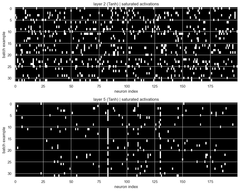

Here the x-axis is the neuron index and the y-axis is the batch example. White pixels are activations with:

This plot is better than a single percentage because it preserves the structure. If we see a full vertical white stripe, that neuron is saturated for almost every example in the batch. That would be a bad sign. If instead we see sparse white pixels, then some examples are saturating but the whole layer is not dead.

In this run, the first Tanh layer is still more saturated than the second one. So BatchNorm helped us control the signal, but it did not magically remove all saturation.

Activation distributions

The saturation map is useful, but I also want the distribution view. The histogram tells us where the mass of the activations is.

# Inspect activation distributions layer by layer
tanh_layers = [(i, layer) for i, layer in enumerate(layers[:-1]) if isinstance(layer, Tanh)]

n = len(tanh_layers)
plt.figure(figsize=(4 * n, 3))

for k, (i, layer) in enumerate(tanh_layers, 1):
    t = layer.out.detach().view(-1)

    mean = t.mean().item()
    std = t.std().item()
    sat = (t.abs() > 0.97).float().mean().item() * 100

    print(f'layer {i:2d} ({layer.__class__.__name__:>10s}) | mean {mean:+.2f} | std {std:.2f} | saturated {sat:.2f}%')

    plt.subplot(1, n, k)
    plt.hist(t.tolist(), bins=40, density=True)
    plt.title(f'layer {i}')
    plt.xlabel(f'μ={mean:+.2f}, σ={std:.2f}\nsat={sat:.1f}%')
    plt.ylim(bottom=0)

plt.suptitle('Activation distributions by layer')
plt.tight_layout()

layer  2 (      Tanh) | mean -0.01 | std 0.74 | saturated 19.19%
layer  5 (      Tanh) | mean -0.01 | std 0.64 | saturated 7.50%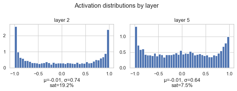

This confirms the same story. The means are close to zero, which is good. But the first layer has a larger standard deviation and more mass close to -1 and 1, so it has more saturated activations.

This is the kind of plot that makes the problem visible: we are not just saying "maybe tanh saturates". We can actually inspect where and how much it is happening.

Gradient distributions

Now we look at the backward pass.

After loss.backward(), each layer output has a gradient. For the Tanh layers, this tells us the gradient signal that is flowing backward through those activations:

# Inspect gradient distributions layer by layer
# We want gradients that are not collapsed to zero and not exploding.
tanh_layers = [(i, layer) for i, layer in enumerate(layers[:-1]) if isinstance(layer, Tanh)]

n = len(tanh_layers)
plt.figure(figsize=(4 * n, 3))

for k, (i, layer) in enumerate(tanh_layers, 1):
    t = layer.out.grad.detach().view(-1)

    mean = t.mean().item()
    std = t.std().item()

    print(f'layer {i:2d} ({layer.__class__.__name__:>10s}) | mean {mean:+.3e} | std {std:.3e}')

    plt.subplot(1, n, k)
    plt.hist(t.tolist(), bins=40, density=True)
    plt.title(f'layer {i}')
    plt.xlabel(f'μ={mean:+.1e}, σ={std:.1e}')
    plt.ylim(bottom=0)

plt.suptitle('Gradient distributions by layer')
plt.tight_layout()

layer  2 (      Tanh) | mean -3.638e-12 | std 3.133e-03
layer  5 (      Tanh) | mean -2.237e-05 | std 5.294e-03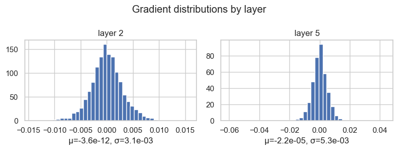

The mean is close to zero, and that is not a problem. Gradients have signs, so positive and negative values can cancel.

The more interesting quantity here is the standard deviation. If the gradient distribution is collapsed almost exactly at zero, the layer is not receiving a useful learning signal. If it is extremely wide, then the backward signal may be unstable.

So here I do not want "large variance" in an absolute sense. I want visible, non-collapsed variance: gradients should carry information, but not explode.

Weight gradient distributions

Finally, we inspect the gradients of the parameters themselves.

For each weight matrix, we plot the distribution of its gradients and compute:

This is a scale-aware diagnostic. A gradient with standard deviation 0.01 may be big or small depending on the scale of the parameter it is updating. So we compare gradient scale against weight scale.

# Inspect weight gradient distributions parameter by parameter
weight_params = [(i, p) for i, p in enumerate(parameters) if p.ndim == 2]

n = len(weight_params)
plt.figure(figsize=(8, 3 * n))

for k, (i, p) in enumerate(weight_params, 1):
    t = p.grad.detach().view(-1)

    mean = t.mean().item()
    std = t.std().item()
    ratio = (p.grad.std() / p.std()).item()

    print(f'weight {tuple(p.shape)!s:>12s} | mean {mean:+.3e} | std {std:.3e} | grad:data ratio {ratio:.3e}')

    plt.subplot(n, 1, k)   # one below the other
    plt.hist(t.tolist(), bins=40, density=True)
    plt.title(f'param {i} - shape {tuple(p.shape)}')
    plt.xlabel(f'μ={mean:+.1e}, σ={std:.1e}, ratio={ratio:.1e}')
    plt.ylim(bottom=0)

plt.suptitle('Weight gradient distributions')
plt.tight_layout()

weight     (27, 10) | mean +3.311e-10 | std 1.384e-02 | grad:data ratio 1.252e-02
weight    (30, 200) | mean +1.307e-05 | std 7.136e-03 | grad:data ratio 1.838e-02
weight   (200, 200) | mean +1.558e-05 | std 4.308e-03 | grad:data ratio 2.301e-02
weight    (200, 27) | mean +2.208e-11 | std 1.813e-02 | grad:data ratio 8.428e-02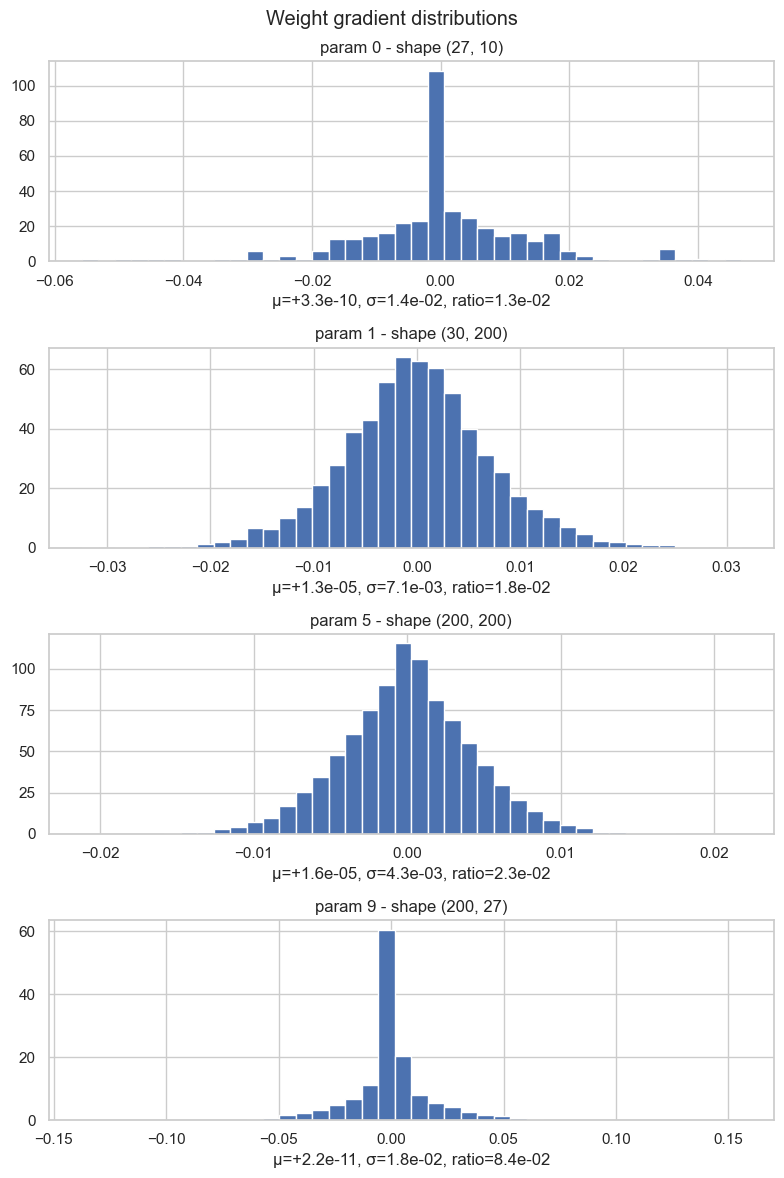

One important detail: this ratio tells us how large the gradient is compared to the weight. But during SGD the weight is not updated with the raw gradient. It is updated with the learning-rate-scaled gradient:

So if we want to know how much the weight really moves, we have to include the learning rate:

For example, if:

weight std    = 1
gradient std  = 0.01
learning rate = 0.01

then:

grad:data ratio   = 0.01 / 1 = 1e-2
update:data ratio = (0.01 * 0.01) / 1 = 1e-4

So the plot tells us how strong the raw gradient signal is. To understand how much the parameters really move after one SGD step, we also have to multiply by the learning rate.

This is the intuition I want from this plot:

• if the ratio is too small, the weights barely move
• if the ratio is too large, the weights are being hit too aggressively
• if one layer is very different from the others, that layer deserves attention

So these plots are not just decoration. They are the basic instruments I want before trusting a training run: loss curve, activation saturation, activation distribution, gradient distribution, and parameter update scale.

Conclusion & Sources

The main point of this post is that a neural network is not just a stack of matrix multiplications followed by loss.backward().

It is also a system that moves distributions forward and gradients backward. If the distributions are badly scaled, the nonlinearities saturate. If the gradients collapse, the model does not learn. If the updates are too large, training becomes unstable. The loss curve shows the final symptom, but the statistics of activations, gradients, and updates show the mechanism.

So the intuition I want to keep is simple: before changing architectures randomly, inspect the signal. Look at means, variances, saturation, gradient distributions, and update ratios. These plots are not advanced tooling; they are the minimum instrumentation needed to understand if the network is actually trainable.

Main practical reference:

• Andrej Karpathy, Neural Networks: Zero to Hero, especially the makemore lectures on activations, gradients, BatchNorm, and manual backpropagation.

Background math and signal/statistics intuition:

• Steven W. Smith, The Scientist and Engineer's Guide to Digital Signal Processing.
• Random variable.
• Bessel correction.
• Law of large numbers.
• Central limit theorem.

Papers cited:

• Yann LeCun, Leon Bottou, Genevieve B. Orr, Klaus-Robert Müller, Efficient BackProp, 1998.
• Xavier Glorot, Yoshua Bengio, Understanding the difficulty of training deep feedforward neural networks, AISTATS 2010.
• Kaiming He, Xiangyu Zhang, Shaoqing Ren, Jian Sun, Delving Deep into Rectifiers: Surpassing Human-Level Performance on ImageNet Classification, 2015.
• Sergey Ioffe, Christian Szegedy, Batch Normalization: Accelerating Deep Network Training by Reducing Internal Covariate Shift, 2015.
• Jimmy Lei Ba, Jamie Ryan Kiros, Geoffrey E. Hinton, Layer Normalization, 2016.
• Kaiming He, Xiangyu Zhang, Shaoqing Ren, Jian Sun, Deep Residual Learning for Image Recognition, 2015.
• Nitish Srivastava, Geoffrey Hinton, Alex Krizhevsky, Ilya Sutskever, Ruslan Salakhutdinov, Dropout: A Simple Way to Prevent Neural Networks from Overfitting, JMLR 2014.
• Hongyi Zhang, Yann N. Dauphin, Tengyu Ma, Fixup Initialization: Residual Learning Without Normalization, 2019.