Engineering MovHex: Modeling and Optimizing a Dynamic Hex-Grid Router in C

1. Introduction

This post is a technical walkthrough of MovHex, my project for Algorithms and Principles of Computer Science at Politecnico di Milano.

The assignment: build a routing engine over a rectangular map of hexagons. The program must support four commands:

1. init — create or reinitialize the map
2. change_cost — update hexagon costs within a hexagonal radius
3. toggle_air_route — add or remove a directed air route
4. travel_cost — answer shortest-path queries

Concretely, the program must accept the following command formats:

init <n_columns> <n_rows>
change_cost <x> <y> <v> <radius>
toggle_air_route <x1> <y1> <x2> <y2>
travel_cost <xp> <yp> <xd> <yd>

where:

• n_columns, n_rows define the size of the rectangular hex map
• x, y identify a hexagon using the specification's coordinate system
• v is the signed update applied by change_cost
• radius is the positive hex-distance radius of the update
• x1, y1 are the source coordinates of a directed air route
• x2, y2 are the destination coordinates of a directed air route
• xp, yp are the source coordinates of a shortest-path query
• xd, yd are the destination coordinates of a shortest-path query

At first glance this looks like "implement Dijkstra on a graph." In practice, the real difficulty is in the interaction between hex geometry, mutable state, and performance constraints.

The verifier for the course included explicit thresholds for 30 cum laude:

• execution time below 10 seconds
• memory usage below 26 MiB

My final version meets both thresholds.

Correctness alone was not enough. The solution had to be modeled carefully, implemented safely in C, and then profiled and specialized until it was fast enough.

Whenever I show code in this post, I show lightly reformatted excerpts from the final main.c in the repository. If a block contains ..., that means omitted lines, not rewritten logic.

2. The Problem, as the Specification Defines It

The official statement describes a rectangular tiling of equal-sized hexagons. Hexagons are identified by column first, row second. Indices start from zero, increase left to right and bottom to top. The hexagon (0,1) sits on the upper-right side of (0,0).

That last detail is important: the coordinate system encodes an offset hex layout, and that affects both neighbor generation and distance computation.

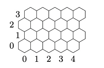
The coordinate system defined by the specification: columns grow left to right, rows grow bottom to top, and (0,1) sits on the upper-right side of (0,0).

Each hexagon stores a natural number in $[0,100]$:

• if positive, it is the ground exit cost of that hexagon
• if 0, the hexagon can still be visited, but it cannot be abandoned — no ground or air departure is possible from it

2.1 init

init n_columns n_rows creates or reinitializes a map of n_rows × n_columns hexagons. All costs are set to 1, no air routes exist. The program responds OK.

2.2 change_cost

change_cost x y v radius updates every hexagon whose hex distance from (x,y) is strictly less than the given radius. The specification calls this distance DistEsagoni and defines it as the minimum number of hexagons traversed to reach the destination from the source, including the destination in the count, ignoring costs, blocked departures, and air routes.

That "including the destination" clause pins the semantics: adjacent hexagons have distance 1, and the hexagon at the center has distance 0 from itself.

In the rest of this post I refer to the same quantity as hexDistance, because that is the name I used while reasoning about the implementation. The formula and the semantics are the same as DistEsagoni in the specification.

The update rule from the specification is:

If I write $d = \operatorname{hexDistance}\big((x_e,y_e),(x,y)\big)$, the additive delta is:

The result is clamped to $[0,100]$. The same update also applies to all outgoing air routes of every affected hexagon. The program responds KO if (x,y) is not a valid hexagon or if radius = 0, otherwise OK.

2.3 toggle_air_route

toggle_air_route x1 y1 x2 y2 adds or removes a directed air route. If the route does not exist, it is created. If it already exists, it is removed.

When a new route is created, its cost is the floor of the average of all already existing outgoing air-route costs from (x1,y1) together with the ground exit cost of (x1,y1). Each hexagon may have at most 5 outgoing air routes. The program responds OK if coordinates are valid and the limit is not exceeded, KO otherwise.

When a route is removed, no cost recalculation happens — the route is simply deleted.

2.4 travel_cost

travel_cost xp yp xd yd asks for the minimum cost of reaching (xd,yd) from (xp,yp). The rules:

1. the exit cost of the destination hexagon is ignored
2. if an air route is used, the ground exit cost of the air route's source hexagon is ignored — you pay the air route's traversal cost instead
3. if source equals destination, the cost is zero regardless of any other factor — even if the source has weight 0
4. responds -1 if coordinates are invalid or if no path exists

That third rule matters. It means a weight-0 hexagon can still produce a valid travel_cost answer when it is both source and destination.

2.5 The Workload Hint

The specification gives one more important clue: in realistic inputs, change_cost and toggle_air_route are rare, while travel_cost is used heavily, and most source/destination pairs concentrate in the same zones.

That hint shaped the whole approach:

• mutations can be more expensive, as long as they are correct
• shortest-path queries are the real hot path
• repeated queries deserve caching, but only with strict invalidation

3. The Engineering Model

The central design question was not "which graph algorithm should I use?" It was: what state does this problem actually require me to store permanently?

The final implementation is built on four decisions:

1. flatten the grid into a 1D array with row-major indexing
2. treat ground adjacency as derived geometry, not stored state
3. store air routes explicitly, because they are the only mutable adjacency
4. keep shortest-path working memory separate from the permanent map

3.1 Permanent State

The permanent map consists of three parallel arrays:

• weight[] (uint8_t) — the ground exit cost of each hexagon, in $[0,100]$
• counter_air_route[] (uint8_t) — the number of outgoing air routes from each node, in $[0,5]$
• air_route[] (uint32_t* per node) — a dynamically allocated array of destination indices for each node, NULL when the node has no outgoing air routes

That is all. No adjacency lists for ground links, no per-route cost fields, no embedded graph metadata.

3.2 Working State

Dijkstra's algorithm needs its own data structures, allocated once after init and reused across every travel_cost query:

• distance[] (uint32_t) — tentative distances from the source, initialized to UINT32_MAX at the start of each run via memset(distance, 0xFF, ...)
• the priority structure (either a binary min-heap or bucket arrays, depending on the compile-time variant)
• a cache hash table for memoizing travel_cost results

This separation matters. Ground neighbors are computed on the fly from coordinates and row parity. Air routes are stored because they mutate. Dijkstra metadata is transient and does not belong inside the map.

3.3 Row-Major Indexing

The mapping between 2D coordinates and the flat index is:

static inline void convert2to1(uint32_t i, uint32_t j, uint32_t COLS, uint32_t *INDEX){
    *INDEX = i * COLS + j;
}

static inline void convert1to2(uint32_t *i, uint32_t *j, uint32_t COLS, uint32_t INDEX){
    *i = INDEX / COLS;
    *j = INDEX % COLS;
}

The original implementation used a struct hex_t containing weight, distance, predecessor, ground-link lists, and air-route lists — all packed into one type. Profiling showed that the struct was too fat for cache lines, and most fields were only needed during Dijkstra. The final architecture is the result of dismantling that struct into flat parallel arrays and removing everything that could be derived instead of stored.

4. The Geometric Core

The first hard problem was not shortest paths. It was getting the geometry right.

A square grid lets you get away with matrix intuition for a long time. A hex grid does not. Neighbor relations depend on row parity, and the specification numbers rows from bottom to top, while most standard hex-grid references assume top-based coordinates. Trying to reason in a matrix-like way immediately produces questions that do not exist on square grids: if I move to the upper-right neighbor, do I stay in the same column or shift? Does that answer change when the row is even?

The external reference that made this click for me was the Red Blob Games guide on hexagonal grids. It gave me the right conceptual model: separate the problem into three coordinate layers instead of trying to make matrix intuition work directly.

4.1 Three Coordinate Layers

1. Specification coordinates: column-first, row-second, rows numbered bottom to top
2. Offset layout: the physical hex grid where row parity shifts neighbor positions — in the specification's convention, odd rows are offset to the right
3. Cube coordinates: a 3D system $(q, r, s)$ subject to the constraint $q + r + s = 0$, which makes distance computation clean and parity-independent

The progression was concrete: matrix intuition broke because it does not account for the row-dependent offset ("lo sfasamento"), and only after recognizing the offset layout explicitly did the cube-coordinate machinery become applicable.

4.2 Parity-Dependent Neighbors

In the offset layout, moving to the upper-right neighbor from a hexagon depends on whether the current row is even or odd. In an even row, the upper-right neighbor is in the same column. In an odd row, it shifts one column to the right.

The final code encodes this as two lookup tables:

const int8_t neighbors_set[2][6][2] = {
    // Even rows (parity 0): (col_offset, row_offset)
    { {-1,+1}, {0,+1}, {+1,0}, {0,-1}, {-1,-1}, {-1,0} },
    // Odd rows (parity 1):
    { {0,+1}, {+1,+1}, {+1,0}, {+1,-1}, {0,-1}, {-1,0} }
};

During Dijkstra, the row parity of the current node selects the correct table, and each of the six neighbors is generated by adding the corresponding offset to the current (col, row) and checking bounds with isinrange. No adjacency list is needed.

4.3 Cube Coordinates and Hex Distance

Hex distance is the core quantity behind change_cost and the geometric model. Computing it directly in offset coordinates is error-prone because the parity-dependent shifts make the arithmetic inconsistent across rows. Cube coordinates solve this.

In cube coordinates, every hexagon is represented as $(q, r, s)$ with the constraint $q + r + s = 0$. The key property: each single hex step changes exactly two of the three coordinates by $\pm 1$ — one increases, one decreases, the third stays the same — so the constraint is always maintained. This means each step adds exactly 2 to the Manhattan distance $|{\Delta q}| + |{\Delta r}| + |{\Delta s}|$. Therefore:

This formula is parity-independent and well-defined regardless of the offset convention, which is the whole point of converting to cube coordinates before computing distance.

4.4 Offset-to-Cube Conversion and the ROWS % 2 Branch

The conversion from offset coordinates to cube depends on whether the layout is odd-r (odd rows shifted right) or even-r (even rows shifted right). The formulas from the Red Blob Games model are:

• odd-r: $q = \text{col} - \lfloor(\text{row} - \text{parity}) / 2\rfloor$,   $r = \text{row}$,   $s = -q - r$
• even-r: $q = \text{col} - \lfloor(\text{row} + \text{parity}) / 2\rfloor$,   $r = \text{row}$,   $s = -q - r$

where $\text{parity} = \text{row} \bmod 2$. The only difference between the two is a single sign flip in the $q$ computation: +parity for even-r, -parity for odd-r. Getting that sign wrong produces plausible-looking results that silently fail on specific row parities.

Now the complication. The specification numbers rows from the bottom. The cube-coordinate formulas assume top-based numbering. Before converting, the code flips the row:

This flip inverts parity when $\text{ROWS} - 1$ is odd (i.e., when ROWS is even):

The consequence:

• if ROWS is odd, $\text{ROWS} - 1$ is even, parity is preserved → the grid remains odd-r after flipping → use the odd-r formula ($-\text{parity}$)
• if ROWS is even, $\text{ROWS} - 1$ is odd, parity inverts → the grid becomes even-r after flipping → use the even-r formula ($+\text{parity}$)

That is the real reason the final code branches on ROWS % 2:

if(ROWS % 2 == 0){
    i1 = (ROWS - 1) - i1;
    i2 = (ROWS - 1) - i2;

    int8_t parity1 = i1 % 2;
    int8_t parity2 = i2 % 2;
    int32_t q1 = j1 - ((i1 + parity1)/2);   // even-r
    int32_t q2 = j2 - ((i2 + parity2)/2);
    ...
}else{
    i1 = (ROWS - 1) - i1;
    i2 = (ROWS - 1) - i2;

    int8_t parity1 = i1 % 2;
    int8_t parity2 = i2 % 2;
    int32_t q1 = j1 - ((i1 - parity1)/2);   // odd-r
    int32_t q2 = j2 - ((i2 - parity2)/2);
    ...
}

Both branches then compute $s = -q - r$ and return $(|q_1-q_2|+|r_1-r_2|+|s_1-s_2|)/2$.

If the even-r/odd-r choice is inverted, or if the row flip is omitted, the distance function produces results that look correct on many test cases but fail systematically on whole classes of inputs where the row parity changes the expected geometry.

5. The Invariant That Simplifies Air Routes

The final representation stores no per-route cost. Each air route is just a destination index. This is possible because of an invariant that holds throughout execution.

Invariant: all outgoing air routes from the same source $u$ always have the same cost, and that cost equals $\operatorname{weight}[u]$.

Proof by induction on the sequence of operations:

1. First air route from $u$: there are no existing air routes. The cost is $\lfloor \operatorname{weight}[u] / 1 \rfloor = \operatorname{weight}[u]$.
2. Inductive step (toggle_air_route): suppose all $k$ existing outgoing air routes from $u$ have cost $\operatorname{weight}[u]$. The new route's cost is $\lfloor (k \cdot \operatorname{weight}[u] + \operatorname{weight}[u]) / (k + 1) \rfloor = \operatorname{weight}[u]$.
3. Preservation through change_cost: the specification says the same update formula applies both to $\operatorname{weight}[u]$ and to all outgoing air routes of $u$. The delta $\Delta(d) = \lfloor v \cdot \max(0, (r - d)/r) \rfloor$ depends only on the distance from the pivot and the parameters $v$ and $r$ — not on the current cost. So weight and every air-route cost receive the same integer delta. After clamping to $[0,100]$, they remain equal.

The consequence: the effective traversal cost of an air move from $u$ is always $\operatorname{weight}[u]$, which is the same as the ground exit cost. The code stores only destination indices:

air_route[index1][*counter_air_route] = index2;
*counter_air_route += 1;

And the shortest-path code uses currweight for both ground and air moves:

// Ground links
new_distance = currdistance + currweight;
...
// Air links
uint32_t neighbor = air_route[i];
new_distance = currdistance + currweight;

This invariant also simplifies change_cost: since air-route costs are implicit in weight[], the function only needs to update the weight array. The air-route cost update mandated by the specification is automatically satisfied.

6. change_cost in the Final Implementation

change_cost is a geometric enumeration problem, not a traversal problem.

An earlier implementation used a queue-based expansion with a visited array — start from the pivot, expand to neighbors, track distance, stop at the radius. It was correct, but profiling showed insert_neighbors was a major bottleneck: expanding neighbors iteratively through linked lists was expensive, especially for large radii.

The final implementation starts from geometry instead. Once the pivot has been converted into cube coordinates, the code iterates directly over all cube offsets inside the hexagonal region:

for (int32_t q2 = -radius; q2 <= radius; q2++) {
    int32_t r2_start = max(-radius, -q2 - radius);
    int32_t r2_end = min(radius, -q2 + radius);
    for (int32_t r2 = r2_start; r2 <= r2_end; r2++) {
        int32_t qc = q1 + q2;
        int32_t rc = r1 + r2;
        ...
        uint32_t distance = hex_distance(j1, i1, j2, i2, ROWS);
        if(distance >= (uint32_t)radius) continue;
        change_cost_hex(weight, index, distance, v, radius);
    }
}

The nested loop directly enumerates all cube coordinates $(q_c, r_c, s_c)$ such that $|q_2| + |r_2| + |s_2| \le 2 \cdot \text{radius}$ (the hexagonal region around the pivot). The r2_start/r2_end bounds enforce the cube constraint $q + r + s = 0$ implicitly — they restrict $r_2$ so that $s_2 = -q_2 - r_2$ stays within $[-\text{radius}, +\text{radius}]$.

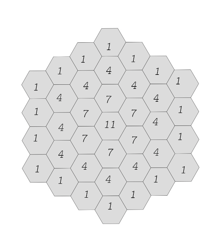
Hexagons at the same hex distance from the center receive the same update delta, so the effect propagates by hex-distance layers.

Each candidate is converted back to grid coordinates, bounds-checked, and then updated with the weighted delta:

int32_t compute_weighted_value(float v, float radius, float distance) {
    float normalized = (radius - distance) / radius;
    float clamped = fmaxf(0.0f, normalized);
    float weighted = v * clamped;
    return (int32_t)floorf(weighted);
}

The update clamps the result to $[0,100]$:

void change_cost_hex(uint8_t *weight, uint32_t index, uint32_t distance,
                     int8_t v, int32_t radius)
{
    int32_t new_weight = compute_weighted_value(v, radius, distance);
    int32_t sum = weight[index] + new_weight;
    if(sum < 0) sum = 0;
    if(sum > 100) sum = 100;
    weight[index] = (uint8_t) sum;
}

7. travel_cost and the Dijkstra Implementations

7.1 The Graph Model

At the modeling level, the problem is a sparse directed graph with nonnegative integer edge weights:

• each hexagon is a node
• ground adjacency contributes up to 6 outgoing edges, derived on the fly from coordinates and row parity
• air routes contribute up to 5 additional outgoing edges, read from air_route[]
• all effective edge weights equal weight[source] (from the invariant in Section 5)
• weights are bounded integers in $[0, 100]$

All edge weights are nonnegative, so Dijkstra's algorithm is the correct base choice. The final code keeps two implementations behind the compile-time flag DIJKSTRA_IMPL: 0 for binary min-heap, 1 for weight-sorted buckets. The default build uses the second.

7.2 Common Structure

Both Dijkstra variants share the same relaxation logic. For the currently visited node, the code computes its row parity via convert1to2, then iterates over all 6 ground neighbors (using neighbors_set[parity]) and all air-route destinations. For each reachable neighbor:

// Ground links
for(int8_t i = 0; i < 6; i++){
    int32_t sx2 = (int32_t)x1 + neighbors_set[parity][i][0];
    int32_t sy2 = (int32_t)y1 + neighbors_set[parity][i][1];
    if(!isinrange(sy2, sx2, ROWS, COLS)) continue;
    ...
    new_distance = currdistance + currweight;
    if(new_distance < distance[neighbor_index]){
        // relax
    }
}
// Air links
for(int8_t i = 0; i < counter_air_route[hexindex_visiting]; i++){
    uint32_t neighbor = air_route[i];
    new_distance = currdistance + currweight;
    if(new_distance < distance[neighbor]){
        // relax
    }
}

Both ground and air relaxation use currdistance + currweight as the candidate distance. The invariant from Section 5 is what makes this correct for air routes: the air-route traversal cost is always equal to the source node's weight.

Both variants handle weight == 0 the same way: a hexagon with zero weight can be visited (its distance is set during relaxation from a neighbor) but it cannot be departed from — its neighbors are never relaxed through it. This directly implements the specification rule that a zero-cost hexagon "cannot be abandoned but can be visited."

Both variants use early exit: once the destination is extracted from the priority structure, the algorithm terminates. Dijkstra's optimality guarantee ensures that at that point its distance is final, so there is no need to continue.

Both variants also handle travel_cost bookkeeping the same way:

if((i1 == i2) && (j1 == j2)){
    *COST = 0;
    return 1;
}
...
if(find_cost(hash_table, index1, index2, COST) == 1){
    if(*COST == UINT32_MAX) return -1;
    return 1;
}
...
// Run Dijkstra
*COST = distance[index2];
insert_cost(hash_table, index1, index2, COST);
if(distance[index2] == UINT32_MAX) return -1;
return 1;

The source-equals-destination check happens before anything else. Then the cache is queried. Only if both miss does Dijkstra run. After the run, the result is cached and returned — including UINT32_MAX for unreachable destinations, so repeated misses also avoid recomputation.

7.3 Binary Min-Heap Variant (DIJKSTRA_IMPL 0)

The heap variant uses a standard binary min-heap with an explicit position-tracking array.

Each heap entry is a heap_block_t:

typedef struct heap{
    uint32_t distance;
    uint32_t hexnumber;
}heap_block_t;

The implementation detail that makes this work is min_heap_index[] (int32_t per node), which tracks every node's state with respect to the heap using three distinct values:

• -1 (initialized via memset(0xFF)): the node has never been inserted into the heap
• valid index (≥ 0): the node is currently in the heap at that position
• INT32_MAX: the node has been popped and must not be reinserted (settled)

This three-state tracking is what allows relax_neighbor to distinguish between insertion and decrease-key without a separate settled array:

static inline void relax_neighbor(heap_block_t *min_heap, uint32_t *distance,
    int32_t *min_heap_index, uint32_t *heap_size,
    uint32_t neighbor_index, uint32_t new_distance)
{
    if(min_heap_index[neighbor_index] == -1){
        // Never seen → insert into heap
        distance[neighbor_index] = new_distance;
        min_heap[*heap_size].distance = new_distance;
        min_heap[*heap_size].hexnumber = neighbor_index;
        min_heap_index[neighbor_index] = *heap_size;
        *heap_size += 1;
        bubble_up(min_heap, min_heap_index[neighbor_index], min_heap_index);
    }else if(min_heap_index[neighbor_index] != INT32_MAX){
        // Currently in heap → decrease-key
        distance[neighbor_index] = new_distance;
        min_heap[min_heap_index[neighbor_index]].distance = new_distance;
        bubble_up(min_heap, min_heap_index[neighbor_index], min_heap_index);
    }
    // If INT32_MAX → already settled, skip
}

pop_min extracts the root, moves the last heap element to position 0, calls min_heapify to restore the heap property, and marks the popped node as INT32_MAX in min_heap_index. Both bubble_up and min_heapify update min_heap_index on every swap, so the mapping stays consistent.

The initialization allocates the heap and index arrays once in main() after init, and each Dijkstra run resets them with memset:

memset(distance, 0xFF, ROWS*COLS * sizeof(uint32_t));
memset(min_heap_index, 0xFF, (ROWS*COLS)*sizeof(int32_t));

The complexity is $O((V + E) \log V)$. Since each hexagon has at most 11 outgoing edges (6 ground + 5 air), $E = O(V)$, so the total is $O(V \log V)$.

7.4 Weight-Sorted Bucket Variant (DIJKSTRA_IMPL 1)

The bucket variant exploits the fact that edge weights are bounded integers in $[0, 100]$.

The idea comes from Dial's algorithm: instead of a heap, use a circular array of 101 buckets indexed by distance % 101. Since the maximum single-edge weight is 100, all active (unprocessed) entries fit within a window of 101 consecutive distance values at any point during execution. Scanning buckets in order from the current index guarantees that entries are processed in nondecreasing distance order.

Each bucket is a buckets_t:

typedef struct buck{
    uint32_t *nodes;  // node indices
    uint32_t *keys;   // distances at insertion time
    int32_t size;     // total entries pushed
    int32_t cursor;   // next entry to pop
    int32_t maxdim;   // current allocation capacity
}buckets_t;

Each bucket stores two parallel arrays — nodes[] and keys[] — instead of an array of structs. This was a deliberate choice driven by the same principle that led to dismantling hex_t: keeping related data types contiguous for better cache behavior during sequential scans.

The relaxation function is much simpler than the heap variant — it just pushes a new entry into the appropriate bucket:

static inline void relax_neighbor_weight_sort(buckets_t *bucket, uint32_t key,
    uint32_t hexindex, uint32_t *tobeprocessed, uint32_t *distance)
{
    distance[hexindex] = key;
    push(bucket, hexindex, key, tobeprocessed);
}

The caller selects the bucket as buckets[new_distance % 101]. This means the same node can appear in multiple buckets with different distances (a lazy approach). The algorithm handles this with stale-entry detection at pop time:

pop(&buckets[idx], &tobeprocessed, &hexindex_visiting, &key);
if(hexindex_visiting == UINT32_MAX){
    idx = (idx+1) % 101;
    continue;
}
...
if (key != currdistance)       continue;  // stale entry — distance was improved since insertion
if (settled[hexindex_visiting]) continue;  // already finalized
if (hexindex_visiting == DST)  break;     // early exit — even if weight is 0
if (currweight == 0)           continue;  // cannot depart from this node

The stale-entry check (key != currdistance) is necessary because a node's best distance may have been improved after this entry was pushed — the old entry remains in the bucket but is no longer valid. The settled[] array (uint8_t per node, zeroed at the start of each run) tracks finalized nodes. The early-exit check comes before the weight check: the destination's distance is already final when it is popped, and its exit cost is ignored by the specification, so there is no reason to continue regardless of its weight.

The bucket scanning loop advances idx = (idx+1) % 101 whenever a bucket is exhausted, cycling through the circular array. The push operation doubles the bucket's allocation when full (realloc to 2 * maxdim). The pop operation resets cursor and size to 0 when the cursor catches up to size, reclaiming the bucket for reuse.

The amortized complexity is $O(V + E + C \cdot V)$ where $C = 101$. Since $E = O(V)$ and $C$ is a constant, this simplifies to $O(V)$ for this problem — eliminating the $\log V$ factor from heap operations.

7.5 Measured Results

• Binary-heap Dijkstra: 8.5 s, 9.6 MiB
• Weight-sorted bucket Dijkstra: 4.4 s, 9.0 MiB

Both satisfy the 30L thresholds. The bucket variant nearly halves the execution time because it replaces $O(\log V)$ heap operations with $O(1)$ bucket insertions and amortized scanning.

8. Caching Repeated Queries

The specification hints that travel_cost will be called frequently and that queries concentrate in the same zones. That made caching worth implementing.

The final strategy is strict:

• exact memoization on (source, destination)
• hash-table lookup before running Dijkstra
• full cache invalidation after every successful init, change_cost, or toggle_air_route
• unreachable destinations cached as UINT32_MAX, so repeated misses also avoid recomputation

There is no partial invalidation. The graph is dynamic and correctness is easy to lose with selective invalidation schemes. Full flush on mutation is simple and trustworthy.

The cache is a 256-bucket hash table with separate chaining. The key is the ordered pair (src, dst): first I combine the two indices with a mixing function using large primes, then I hash the result using Knuth's multiplicative method and take the top 8 bits as the bucket index:

uint32_t combine(uint32_t src, uint32_t dst){
    return src * 73856093u ^ dst * 19349663u;
}

static inline uint32_t hash(uint32_t k) {
    uint64_t prod = (uint64_t)k * ALPHA_FIXEDPOINT;
    uint32_t frac = (uint32_t)prod;
    return frac >> 24;
}

ALPHA_FIXEDPOINT is 2654435769u, the fixed-point representation of Knuth's suggested constant $(\sqrt{5}-1)/2$. The shift by 24 bits produces an 8-bit index in $[0, 255]$.

Invalidation after a successful mutation flushes the entire table:

if(change_cost(weight, args, ROWS, COLS) == 1){
    printf("OK\n");
    free_hash_table(hash_table);
}

The same pattern is used after init and toggle_air_route.

9. Profiling and the Optimization Sequence

Once the code was correct, profiling determined the optimization path. This was not guesswork — I used xctrace (Time Profiler) and Cachegrind at multiple stages.

One Cachegrind snapshot from an earlier version showed:

These bottlenecks were not all of the same kind:

• Heap maintenance (min_heapify + pop_min + bubble_up totaling ~52%) dominated inside repeated shortest-path queries. The $\log V$ cost per operation was being paid on every node extraction and every decrease-key.
• Neighbor expansion (insert_neighbors at ~10%) was expensive in the traversal-based change_cost — it was walking linked lists to find neighbors instead of computing them directly.
• Pointer-heavy structures (the original hex_t struct with embedded linked lists for ground links and air routes) were hurting cache locality. The _int_malloc and _int_free entries in the full Cachegrind output confirmed that dynamic allocation overhead was nontrivial.

That breakdown pushed a specific sequence of redesigns:

1. change_cost: traversal to geometric enumeration. The queue-based expansion with visited arrays was replaced with the direct cube-offset iteration shown in Section 6. The traversal version spent most of its time in insert_neighbors; the geometric version eliminated that function entirely.
2. Linked lists to arrays. Ground links and air routes were moved from linked lists to compact arrays. Sequential array access is fundamentally faster than pointer chasing through scattered heap-allocated nodes. The Cachegrind data confirmed that _int_malloc and _int_free were contributing nontrivial overhead from the linked-list allocations.
3. Struct hex_t dismantled into parallel arrays. Weight, distance, heap index, air routes, and counters became separate flat arrays. This let the hot loop in Dijkstra touch only the data it actually needed per iteration instead of pulling an entire multi-field struct into cache.
4. Separation of permanent and working state. Distance and heap arrays were moved out of the per-node struct entirely, allocated once in main() and reused across queries. The permanent map shrank to just weight[], counter_air_route[], and air_route[].
5. Bucket-based Dijkstra (post-submission refinement). The bounded-weight property $[0, 100]$ made the binary heap overqualified. The 101-bucket Dial's variant eliminated the $\log V$ factor from priority operations, nearly halving execution time.

Every optimization that worked was a removal of unnecessary state, not an addition of clever machinery.

10. Why the Final Design Fits the Problem

The final implementation works because the representation, the invariants, and the hot-path optimizations are aligned with the structure of the assignment:

• geometry is handled through an explicit offset/cube model, not square-grid intuition
• ground adjacency is derived on the fly because it never mutates
• air routes are stored explicitly because they are the only mutable adjacency
• air-route costs are implicit in weight[] because the specification guarantees a stable invariant
• change_cost operates by geometric enumeration in cube space because the command is defined by hex distance
• travel_cost is backed by Dijkstra with a three-state index tracker (heap variant) or stale-entry tolerance (bucket variant), with early exit on the destination
• repeated queries are cached with exact (src, dst) memoization and full invalidation on mutation
• bounded weights in $[0, 100]$ justify replacing a generic $O(\log V)$ heap with a constant-time bucket structure

The performance gain did not come from switching to a fancier shortest-path algorithm alone. It came mostly from making the data layout match the actual geometry, mutability, and bounded-weight structure of the problem: smaller permanent state, fewer cache misses, less pointer chasing, and less unnecessary memory traffic in the hot path.