From Self-Attention to a Small GPT

Introduction

This post is a continuation of my notes on language modeling, adapted from the notes that I took while studying the topic. The goal is to start from the simplest character-level model,as explained in other posts, and then build the core ideas that lead to a small GPT-style transformer.

The main focus is the attention mechanism: why it is needed, how causal self-attention works, and how it fits inside a transformer block.

The path is:

1. tokenization and the next-character prediction task
2. batching fixed-length context windows
3. the bigram model as the simplest language model
4. why tokens need to communicate
5. causal averaging as the first intuition for attention
6. query, key, and value vectors
7. scaled dot-product self-attention
8. multi-head attention
9. feed-forward layers, residual connections, dropout, and layer normalization

The objective is to understand what each piece is doing.

Language Modeling Setup

A language model predicts the next token given the previous tokens:

In this project the model is character-based, so every character is mapped to an integer. This keeps the vocabulary small and makes the implementation easier to inspect.

There are more powerful tokenizers, for example:

• The Google's one: SentencePiece
• The OpenAI's one: tiktoken

but for a first implementation a character-level tokenizer is enough.

If the vocabulary is:

chars = sorted(list(set(text)))
stoi = {ch: i for i, ch in enumerate(chars)}
itos = {i: ch for ch, i in stoi.items()}

then encoding and decoding are just table lookups:

encode = lambda s: [stoi[c] for c in s]
decode = lambda xs: "".join(itos[i] for i in xs)

Words&Vectors

The model never sees strings directly. It sees tensors of integer token ids.

This is the first important shift: for the model, characters are not characters. They are numbers. But a raw integer id is not a good representation by itself, because the number 10 is not “more character” than the number 3. The id is only an index.

For this reason we use an embedding table. Each token id selects a learned vector, and that vector becomes the internal representation of the token.

As humans, we have a strong geometric intuition only up to two or three dimensions. In deep learning, instead, we work with high- dimensional spaces. The idea is that a vector with many dimensions can encode many useful features at the same time.

In a character-level model these features are not necessarily human-readable meanings. The model may learn that some characters behave like vowels, that some often appear after others, or that some are common near word endings. The important point is that the representation is learned from data.

A good way to build intuition for this is to look at pretrained word embeddings. In that case, words with similar meaning often end up close in the embedding space. Classic examples show that relationships such as king - man + woman can point near queen.

Our model is much smaller and works at character level, but the principle is the same: instead of treating tokens as isolated symbols, we map them into vectors that the neural network can modify, combine, and use for prediction.

Before seeing an example, we need another important concept from linear algebra: the standard dot product, also known as the standard inner product.

When we work with a vector space, we can associate it with an inner product, which is a function that takes two vectors and returns a real number:

An inner product must satisfy some properties:

• it is linear in its arguments
• it is symmetric
• it is positive definite, so $\langle v, v \rangle \ge 0$
• $\langle v, v \rangle = 0$ only when $v = 0$

When we work in the standard space $\mathbb{R}^n$, the standard dot product between two vectors

and

is defined as:

So we multiply the entries in the same position and then we sum everything.

There is also a geometric interpretation. If $\|a\|$ and $\|b\|$ are the lengths of the two vectors, then:

where $\theta$ is the angle between the two vectors.

This is important for embeddings because now we have a way to compare two vectors. If two embedding vectors point in a similar direction, then intuitively they are carrying similar information. If they point in very different directions, then they are representing something different.

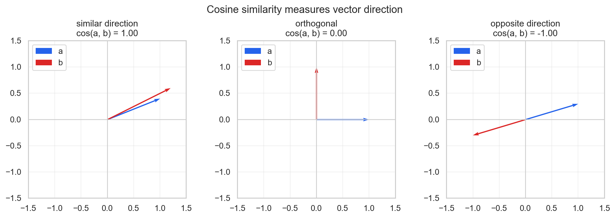
The problem is that the raw dot product also depends on the length of the vectors. So if we want to focus only on the direction, we use cosine similarity:

The value is between $-1$ and $1$:

• if it is close to $1$, the two vectors point in a similar direction
• if it is close to $0$, the two vectors are almost orthogonal
• if it is close to $-1$, the two vectors point in opposite directions

For embeddings, this gives us a practical measure of similarity. If two words have similar meaning, we expect their vectors to have a high cosine similarity.

In the next example, we can use pretrained GloVe embeddings and test this directly with PyTorch.

Reference: GloVe: Global Vectors for Word Representation.

Context Windows and Batches

When training a transformer, we do not push the entire dataset into the model at once. We sample fixed-length chunks.

If block_size = 8, then each row of the batch contains 8 input tokens and 8 target tokens. The target sequence is just the input sequence shifted by one position:

x = data[i:i + block_size]
y = data[i + 1:i + block_size + 1]

So for one row:

x: [18, 47, 56, 57, 1, 58, 46, 43]
y: [47, 56, 57, 1, 58, 46, 43, 1]

This contains multiple training examples at the same time. At position t, the model should predict y[t] using only x[:t+1].

The batch dimension allows parallelization:

def get_batch(split):
    data = train_data if split == "train" else val_data
    ix = torch.randint(len(data) - block_size, (batch_size,))
    x = torch.stack([data[i:i + block_size] for i in ix])
    y = torch.stack([data[i + 1:i + block_size + 1] for i in ix])
    return x, y

The shape is:

x: (B, T)
y: (B, T)

where B is the batch size and T is the context length.

The Bigram Baseline

The simplest neural language model is a bigram model.

It predicts the next token using only the current token:

In PyTorch this can be implemented with an embedding table of shape:

vocab_size x vocab_size

When we pass an integer token id, the embedding table returns the corresponding row. That row contains the logits for the next character.

class BigramLanguageModel(nn.Module):
    def __init__(self, vocab_size):
        super().__init__()
        self.token_embedding_table = nn.Embedding(vocab_size, vocab_size)

    def forward(self, idx, targets=None):
        logits = self.token_embedding_table(idx)

        if targets is None:
            return logits, None

        B, T, C = logits.shape
        logits = logits.view(B * T, C)
        targets = targets.view(B * T)
        loss = F.cross_entropy(logits, targets)
        return logits, loss

The loss is cross entropy. Internally, cross entropy applies softmax to convert logits into probabilities and then computes the negative log likelihood of the correct target.

If the target probability is high, the loss is low. If the target probability is low, the loss is high.

Generation

Generation repeatedly asks the model for the next-token distribution and samples from it.

def generate(self, idx, max_new_tokens):
    for _ in range(max_new_tokens):
        logits, _ = self(idx)
        logits = logits[:, -1, :]
        probs = F.softmax(logits, dim=-1)
        idx_next = torch.multinomial(probs, num_samples=1)
        idx = torch.cat((idx, idx_next), dim=1)
    return idx

At this stage, looking only at the last time step seems wasteful because the model computes logits for all positions. But this structure becomes useful once the model starts using the whole context.

Why Tokens Need to Communicate

The bigram model has a hard limitation: every token is predicted from one previous token only.

This is not enough for language. The meaning of a token depends on the previous context. A token should be able to receive information from previous tokens.

The constraint is causal:

past tokens -> current token
future tokens are hidden

So information can flow from left to right, but not from right to left.

The simplest way to let tokens communicate is to average the previous token vectors.

If x has shape:

(B, T, C)

then for each position t, we want:

This gives each token a "bag of previous words" representation.

Causal Averaging with Matrix Multiplication

The naive implementation is a double loop:

out = torch.zeros_like(x)
for b in range(B):
    for t in range(T):
        xprev = x[b, :t + 1]
        out[b, t] = torch.mean(xprev, 0)

The same operation can be written as matrix multiplication.

We create a lower triangular matrix:

tril = torch.tril(torch.ones(T, T))
wei = tril / tril.sum(1, keepdim=True)
out = wei @ x

The matrix wei contains the averaging weights. Since it is lower triangular, each token can only aggregate information from itself and from previous tokens.

This is the first intuition for attention: each token aggregates information from previous tokens using a weight matrix.

The limitation is that these weights are fixed. They do not depend on the actual content of the tokens.

From Fixed Weights to Data-Dependent Weights

Self-attention makes the aggregation weights data-dependent.

Each token starts with a private representation x that contains:

• token identity
• positional information

Then each token produces three vectors:

• query: what this token is looking for
• key: what this token contains when another token looks at it
• value: what this token will communicate

In code:

key = nn.Linear(n_embd, head_size, bias=False)
query = nn.Linear(n_embd, head_size, bias=False)
value = nn.Linear(n_embd, head_size, bias=False)

Given:

x # (B, T, C)
q = query(x) # (B, T, head_size)
k = key(x)   # (B, T, head_size)
v = value(x) # (B, T, head_size)

we compute the affinity between tokens using the dot product between queries and keys:

wei = q @ k.transpose(-2, -1)

The result has shape:

(B, T, T)

For every token at position i, wei[i, j] tells how much token i wants to receive from token j.

Causal Masking

In language modeling, token i cannot receive information from future tokens.

So we mask the upper triangular part of the attention matrix:

wei = wei.masked_fill(tril == 0, float("-inf"))
wei = F.softmax(wei, dim=-1)

After softmax, every row is a probability distribution over the allowed previous positions.

The output is:

out = wei @ v

So every token receives a weighted sum of the value vectors of previous tokens.

Why We Scale by the Head Size

For a fixed pair of tokens i, j, the raw attention score is:

where:

Assume for intuition that:

and that the components are independent.

For each term:

we have:

and:

The score is a sum of d independent terms:

so:

and the standard deviation grows like:

If d is large, the values entering softmax can become large in magnitude. Then softmax becomes very peaky, often close to a one-hot vector.

To keep the variance stable, we divide by:

The scaled attention score is:

and now:

This is scaled dot-product attention.

A Single Attention Head

Putting the pieces together:

class Head(nn.Module):
    def __init__(self, head_size):
        super().__init__()
        self.key = nn.Linear(n_embd, head_size, bias=False)
        self.query = nn.Linear(n_embd, head_size, bias=False)
        self.value = nn.Linear(n_embd, head_size, bias=False)
        self.register_buffer("tril", torch.tril(torch.ones(block_size, block_size)))
        self.dropout = nn.Dropout(dropout)

    def forward(self, x):
        B, T, C = x.shape
        k = self.key(x)
        q = self.query(x)
        wei = q @ k.transpose(-2, -1) * C**-0.5
        wei = wei.masked_fill(self.tril[:T, :T] == 0, float("-inf"))
        wei = F.softmax(wei, dim=-1)
        wei = self.dropout(wei)
        v = self.value(x)
        out = wei @ v
        return out

There is one important correction in this code: the scaling factor should use the head dimension, not the original embedding dimension. A clearer version is:

wei = q @ k.transpose(-2, -1) * k.shape[-1]**-0.5

The output shape is:

(B, T, head_size)

Each token now carries information aggregated from the previous tokens according to learned, data-dependent weights.

Multi-Head Attention

A single head gives one attention pattern.

Multi-head attention runs several heads in parallel:

class MultiHeadAttention(nn.Module):
    def __init__(self, num_heads, head_size):
        super().__init__()
        self.heads = nn.ModuleList([Head(head_size) for _ in range(num_heads)])
        self.proj = nn.Linear(num_heads * head_size, n_embd)
        self.dropout = nn.Dropout(dropout)

    def forward(self, x):
        out = torch.cat([h(x) for h in self.heads], dim=-1)
        out = self.dropout(self.proj(out))
        return out

If n_embd = 384 and num_heads = 6, then each head can have:

head_size = 384 / 6 = 64

The idea is that different heads can specialize in different relationships between tokens.

Feed-Forward Network

After attention, each token has received information from the previous context.

Then we let each token process its own representation independently with a feed-forward network:

class FeedForward(nn.Module):
    def __init__(self, n_embd):
        super().__init__()
        self.net = nn.Sequential(
            nn.Linear(n_embd, 4 * n_embd),
            nn.ReLU(),
            nn.Linear(4 * n_embd, n_embd),
            nn.Dropout(dropout),
        )

    def forward(self, x):
        return self.net(x)

Attention is the communication step. The feed-forward network is the computation step.

Transformer Block

A transformer block combines:

• communication: multi-head self-attention
• computation: feed-forward network
• residual connections
• layer normalization

class Block(nn.Module):
    def __init__(self, n_embd, n_head):
        super().__init__()
        head_size = n_embd // n_head
        self.sa = MultiHeadAttention(n_head, head_size)
        self.ffwd = FeedForward(n_embd)
        self.ln1 = nn.LayerNorm(n_embd)
        self.ln2 = nn.LayerNorm(n_embd)

    def forward(self, x):
        x = x + self.sa(self.ln1(x))
        x = x + self.ffwd(self.ln2(x))
        return x

The residual connections give gradients a direct path through the network. This is important because the model becomes deep once we stack multiple transformer blocks.

The layer normalization standardizes each token along the feature dimension. In this implementation it is applied before attention and before the feed-forward network.

This is called a pre-norm transformer block.

Small GPT Model

The full model uses:

• token embeddings
• positional embeddings
• stacked transformer blocks
• final layer normalization
• a linear layer that predicts the next token

class GPTLanguageModel(nn.Module):
    def __init__(self):
        super().__init__()
        self.token_embedding_table = nn.Embedding(vocab_size, n_embd)
        self.position_embedding_table = nn.Embedding(block_size, n_embd)
        self.blocks = nn.Sequential(*[Block(n_embd, n_head=n_head) for _ in range(n_layer)])
        self.ln_f = nn.LayerNorm(n_embd)
        self.lm_head = nn.Linear(n_embd, vocab_size)

    def forward(self, idx, targets=None):
        B, T = idx.shape
        tok_emb = self.token_embedding_table(idx)
        pos_emb = self.position_embedding_table(torch.arange(T, device=idx.device))
        x = tok_emb + pos_emb
        x = self.blocks(x)
        x = self.ln_f(x)
        logits = self.lm_head(x)

        if targets is None:
            loss = None
        else:
            B, T, C = logits.shape
            logits = logits.view(B * T, C)
            targets = targets.view(B * T)
            loss = F.cross_entropy(logits, targets)

        return logits, loss

The token embedding tells the model what token it is looking at. The positional embedding tells the model where the token is in the context window.

Without positional embeddings, the transformer has no direct notion of order.

Top-Down View

A compact way to see the full path is:

1. We want to predict the next character.
2. To do that, we represent characters as tokens.
3. Since order matters, we add positional information.
4. To predict well, each token needs information from the previous context.
5. To obtain that information, we use causal self-attention.
6. In self-attention, every token emits a query, a key, and a value.
7. Query-key dot products decide how much information should be taken from each previous token.
8. Values carry the information that is actually aggregated.
9. Multiple heads allow different attention patterns to run in parallel.
10. Feed-forward layers let each token process its own representation.
11. Residual connections and layer normalization make the deep network trainable.

Self-Attention and Cross-Attention

This mechanism is called self-attention because queries, keys, and values all come from the same input x.

In cross-attention, the queries usually come from one sequence, while keys and values come from another sequence.

For example, in an encoder-decoder transformer:

• decoder states produce the queries
• encoder states produce the keys and values

So cross-attention lets one sequence attend to information produced by another sequence.

In a GPT-style decoder-only model, we only use causal self-attention.

Conclusion

The attention mechanism is a learned, data-dependent way to move information between tokens.

The causal mask makes it usable for language modeling because each token can only look at the past. Scaling keeps the softmax numerically well-behaved. Multi-head attention lets the model learn several communication patterns at the same time.

Once attention is combined with feed-forward layers, residual connections, dropout, and layer normalization, we obtain the basic transformer block used in a small GPT.