Deep Dive on a custom GPT architecture

Now that I have covered the fundamentals of neural networks and I have a grasp of how a transformer work, I decided to play around with it, training it over several corpous and see what happens.

The first step, as usual, was to rewrite it from scratch without using the already working out of the box libraries. I like to rebuild it from scratch for remembering that is not something magical, it's just math and scale that play together to obtain something that incredibily work!

For having a solid base that I can fork whenever I want to play around with models and take them for a spin, I decided to create repo that will be the starting point for the experiment, then we clearly need to tweak the details, but the most important thing is the architecture.

Another thing to remember is that you can clearly play with this model even on your laptop, but if you want to start playing also with a bit of scale you'll need a GPU. For my experiment I am using and old pc that I built back in 2020. The specs are not clearly extremely powerful but it's a good starting point. I turned this PC into a server using an Ubuntu LTS distro and then I can connect via SSH through TailScale. The now called server is equipped with 32Gb of RAM and a Ryzen 5 3600, but the fundamental piece is the rx 5600xt. I had to compile a custom release of pytorch for being able to run the code using the GPU as backend, with some strange config now I can run the code just telling pytorch that the device is Cuda.

Before starting to build the architecture I want to dive into the computational cost of inference and training of a model like this one.

Deriving from scratch the computational cost of training and inference

As we know computational cost is usually measured in FLOPs(floating point operations), for example one multiplication is considered 1 flop, the same for addition. Now the goal is to derive a rough mental model of the computational cost for training and inference of an LLM.

We can start from the basics, the fundamental building block is matmul, suppose we want to multiply the following matrices

C = A @ B

where A has shape $MxK$ and B has shape $KxN$ and C has shape $MxN$ . We have to multiply each row of A for each column of B, so we obtain:

FLOPs = 2 * \ K * \ N * M

given that for every row column multiplication we have to perform K multiplication and K-1 sums, we can approximate to 2K, then we have to do that for each column of B and for each row of A.

Now we can extend that reasoning to a classic linear layer:

y = x@w

Nothing that we have not seen yet, it's still a matrix multiplication. Now we can suppose that x has shape $(B,T,C)$ where B is the batch dimension, T is the sequence length and C is the embedding dimension. Then we can suppose that w has dimension $(C,D)$ , mos of the times we have C = D.

We can approach it by thinking that we are executing along the batch dimension in parallel B matmul, we obtain the following:

flops \ linear \ layer = B * 2 * C * T * D = 2 * B * T * D^2

Now we can try to estimate the cost of an attention block. In an attention block we have the following matrices:

x (B, T, C) input
query (C, head_size)
key (C, head_size)
value (C, head_size)

Then we have to perform the following operation, for a single head:

q = x @ query (B, T, head_size)
k = x @ key (B, T, head_size)
v = x @ value (B, T, head_size)
attention = q @ key.transposed() (B,T,head_size) @ (B,head_size,T) -> (B,T,T)
softmax(attention), row-wise over the last dimension -> (B, T, T)
y = attention @ value (B, T, T) @(B, T, head_size) - >(B, T, head_size)

Now we can compute the flops for each step, for this single head:

$flops = 2 \cdot B \cdot C \cdot T \cdot head\_size$
$flops = 2 \cdot B \cdot C \cdot T \cdot head\_size$
$flops = 2 \cdot B \cdot C \cdot T \cdot head\_size$
$flops = 2 \cdot B \cdot head\_size \cdot T^2$
$flops \approx 4 \cdot B \cdot T^2$ (derived below)
$flops = 2 \cdot B \cdot T^2 \cdot head\_size$

Since every real head runs this same computation independently, and there are $h$ of them, the total cost across all heads is simply $h$ times the above. Using $h \cdot head\_size = C$ :

h \cdot \big( \underbrace{6 \cdot B \cdot T \cdot C \cdot head\_size}_{\text{qkv}} + \underbrace{4 \cdot B \cdot T^2 \cdot head\_size}_{\text{scores + weighted sum}} \big) + \underbrace{4 \cdot B \cdot T^2 \cdot h}_{\text{softmax}} = 6BTC^2 + 4BT^2C + 4BT^2h

After the heads are concatenated back into a $(B,T,C)$ tensor, there's one more matmul — the output projection — which is not per-head, so it isn't scaled by $h$ :

flops_{out\_proj} = 2 \cdot B \cdot T \cdot C^2

Adding it in:

\boxed{flops_{attention} = 8 \cdot B \cdot T \cdot C^2 \;+\; 4 \cdot B \cdot T^2 \cdot C \;+\; 4 \cdot B \cdot T^2 \cdot h}

On the softmax cost: Softmax on a row of length $T$ requires: a max-reduction for numerical stability ( $T-1$ comparisons), a subtract-and-exponentiate pass ( $2T$ flops — one subtraction and one exp per element, counting exp as 1 flop by convention), a sum-reduction ( $T-1$ additions), and a final divide ( $T$ divisions). That's $\approx 5T$ flops per row, though $4T$ is the more common rounding in the literature and the two are interchangeable at this level of approximation. There are $B \cdot T$ rows per head (one per query position, per batch element), so one head's softmax costs $\approx 4 \cdot B \cdot T^2$ — independent of $head\_size$ . This is why it has to be added on top of the per-head total above rather than folded into it via the $h \cdot head\_size = C$ substitution: it's the one term whose cost doesn't factor through that product, since it scales with the number of heads (independent softmax calls), not with how wide each head is.

Now it's time to derive the cost of the other fundamental block, the feedforward layer in which usually we have two linear layer and a non-linearity between them. Usually we have that the first linear layer expand by 4 the dimensionality of the input and then we have the non linearity. Then we have the second linear layer that project back to the original dimension:

h = x @ W1 (B, T, C) @ (C, 4C) -> (B, T, 4C)
h = activation(h) (B, T, 4C) -> (B, T, 4C)
y = h @ W2 (B, T, 4C) @ (4C, C) -> (B, T, C)

We already have the formula for a linear layer, so we can reuse it directly for step 1 and step 3.

$flops = 2 \cdot B \cdot T \cdot C \cdot 4C = 8 \cdot B \cdot T \cdot C^2$
activation is elementwise, cost linear in the number of elements ( $B \cdot T \cdot 4C$ ), negligible compared to the matmuls, so we drop it
$flops = 2 \cdot B \cdot T \cdot 4C \cdot C = 8 \cdot B \cdot T \cdot C^2$

Summing:

\boxed{flops_{FFN} = 16 \cdot B \cdot T \cdot C^2}

Notice this is exactly twice the $8 \cdot B \cdot T \cdot C^2$ term from attention (the qkv + output projection part) — the FFN is the more expensive of the two sub-blocks per layer, by a factor of 2, for the standard 4x expansion ratio.

Now we can put together the piece to obtain the computational cost of one of the blocks of the transformer, in which we have the attention layer and the feedfoward network. Usually we stack up a lot of this blocks.

\boxed{flops_{layer} = flops_{attention} + flops_{ffn} = 8 \cdot B \cdot T \cdot C^2 \;+\; 4 \cdot B \cdot T^2 \cdot C \;+\; 4 \cdot B \cdot T^2 \cdot h \;+\;16 \cdot B \cdot T \cdot C^2 }

So at the end we obtain

\boxed{flops_{layer} = 24 \cdot B \cdot T \cdot C^2 \;+\; 4 \cdot B \cdot T^2 \cdot C \;+\; 4 \cdot B \cdot T^2 \cdot h }

Now if we assume to have l layers, one forward pass is going to cost l for $flops_{layer}$ , usually we have also the embedding layer and the final layer of projection over the vocabulary.

The embedding layer is basically a lookup, so we can consider its arithmetic cost equal to zero in this approximation. At the end of the model we also have the language model head, which projects the representation of every token from $C$ to vocab_size. This is another linear layer, so its cost is:

flops_{lm\_head} = 2 \cdot B \cdot T \cdot C \cdot vocab\_size

Even when the language model head shares its weights with the token embedding, we still have to perform this matrix multiplication. Weight tying reduces the number of parameters, not the computational cost of the projection.

Putting together the $l$ transformer layers and the final projection, we obtain the cost of one complete forward pass:

\boxed{flops_{forward} = l \cdot \left(24 \cdot B \cdot T \cdot C^2 + 4 \cdot B \cdot T^2 \cdot C + 4 \cdot B \cdot T^2 \cdot h\right) + 2 \cdot B \cdot T \cdot C \cdot vocab\_size}

Often it is more useful to reason about the cost per token. In one forward pass we process $B \cdot T$ tokens, so we can divide the previous formula by this value:

\boxed{flops_{forward\_per\_token} = 24 \cdot l \cdot C^2 + 4 \cdot l \cdot T \cdot C + 4 \cdot l \cdot T \cdot h + 2 \cdot C \cdot vocab\_size}

This formula makes the two main scaling behaviours more visible. The projections inside the transformer grow quadratically with the embedding dimension $C$ , while the cost of attention over the complete sequence grows quadratically with the context length $T$ .

For training we also have to perform the backward pass. A useful rough approximation is that the backward pass costs around two times the forward pass:

flops_{backward} \approx 2 \cdot flops_{forward}

The complete training cost is then approximately three times the forward cost. Per token we obtain:

\boxed{flops_{training\_per\_token} \approx 72 \cdot l \cdot C^2 + 12 \cdot l \cdot T \cdot C + 12 \cdot l \cdot T \cdot h + 6 \cdot C \cdot vocab\_size}

Custom GPT architecture

Clearly I have not developed from scratch this model architecture, is derived from the original attention paper, plus some other sources, like karpathy's videos and also deep learning books. It's pretty easy, nothing too complicated, I just want to graps the fundamentals, so it's deliberately written in clanky python and pytorch, nothing that must be taken for serious.

You may have already some familiarity with the architecture so you can skip this part if so. For retention I like to plot with tools what I am developing, and in this case I have done a sketch on excalidraw, that in my opinion is very helpful:

architecture

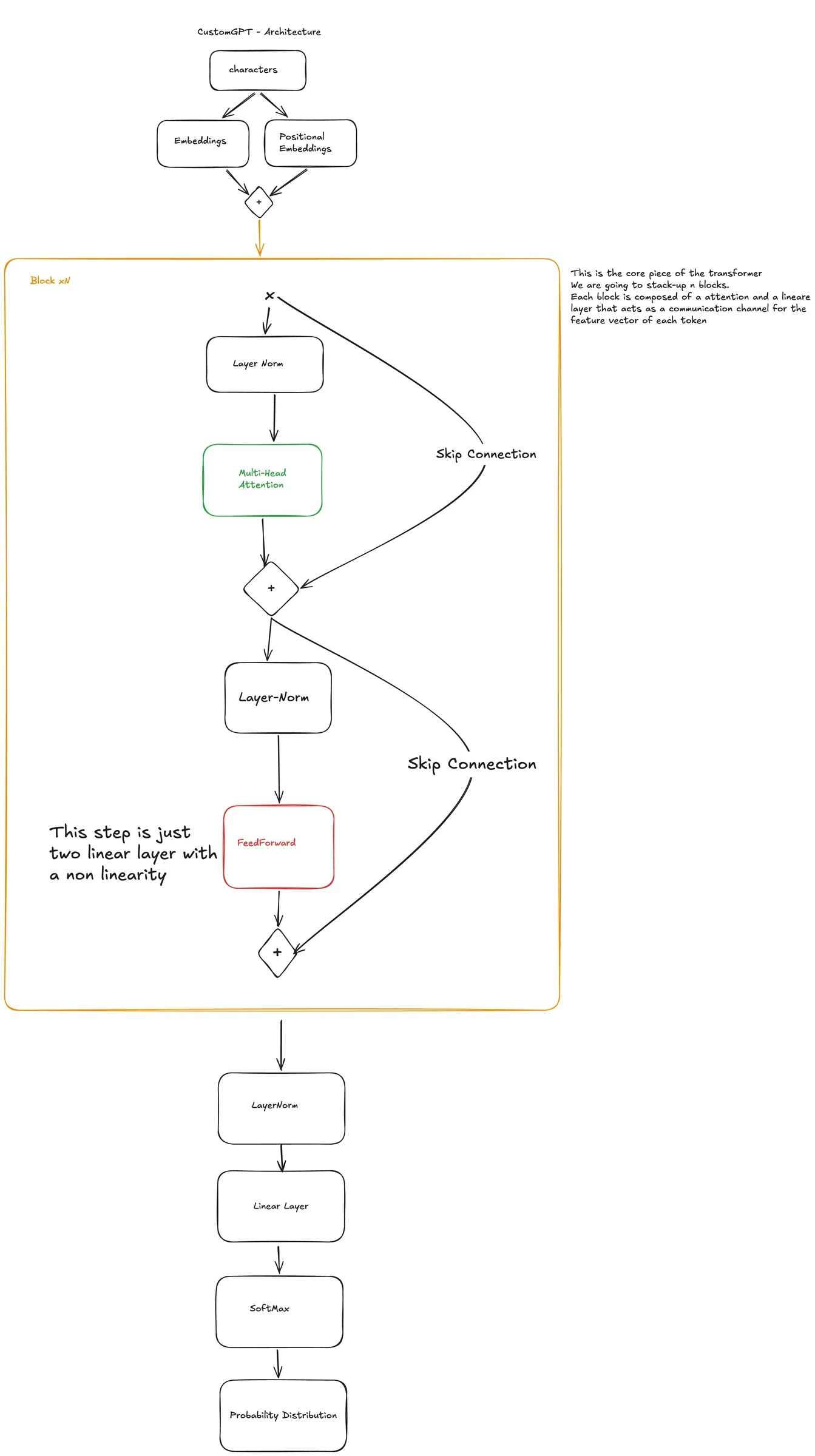
As we have already seen we have the classic transformer block in which we have the attention layer interperse with the ffn layer. We have only a slightly differen thing, that is where we are placing the layer norm, in the paper was after the block, here instead we are placing it before the blocks. It works better there.

You can find it also on GitHub where there is also all the boilerplate for the training and for the inference. I had to use a trick, in which instead of loading all the training set in ram , i had to use a numpy funcitonality to fcreate a pointer to the disk so i do not have crash or OOM during training.

Now we can see some example of this custom gpt at work.

SumGPT

The first experiment is SumGPT, a small model trained to sum two three-digit numbers. The input has a format like 123+456= and the model has to generate the result followed by a newline. I decided to generate the digits of the result in reverse order, because this aligns the carry operation with the autoregressive direction of the model: it can start from the units and then move to tens, hundreds and thousands.

For this task I used a deliberately small configuration, with an embedding size of 128, 4 attention heads, 4 transformer blocks and a context length of 12. The complete operation fits inside this context, so there is no reason to use a larger model. On my GPU the training took around three minutes, and on 1000 randomly generated sums it reached around 99% accuracy.

An interesting thing that I noticed during training was that the loss was not measuring only the ability to perform the sum. The operands before the = sign are generated randomly, so asking the model to predict them introduces a part of the loss that cannot be reduced: there is no pattern that allows it to know which random digit comes next. I fixed this by masking all targets before =, so the cross-entropy only measures the generated result.

This is a small and constrained experiment, but it shows that the architecture can learn an algorithmic pattern and not only the statistical structure of natural language. It also shows how important it is to understand what the loss is actually measuring: a high loss does not always mean that the model is failing at the task we care about.

BookGPT

The second experiment is BookGPT, a character-level language model trained on Italian books. Here the task is more open: given a sequence of characters, the model has to predict the next one and generate prose one character at a time.

The first dataset was composed of 19 books from an Hugging Face dataset, plus I Promessi Sposi. During the experiment I discovered that most of those books were English Gutenberg texts translated automatically into Italian. The corpus contained duplicated fragments, strange sentences and even a book with the wrong title. The model learned these artifacts: the generated text had a recognizable Italian structure, but it also produced many invented words and English names like Sighbury and Mr. Wergomestane.

For this reason I rebuilt the dataset using 15 native Italian works from authors like Manzoni, Verga, Pirandello, Nievo, De Amicis, Deledda and Collodi. The final clean corpus contains around 9.48 million characters and a vocabulary of 140 characters. Every book was split independently into 90% training and 10% validation before concatenating them, to avoid having a validation set biased toward only the last books in the corpus.

I trained three comparable configurations.

The first one was the baseline trained on the old corpus. It had around 852K parameters, an embedding size of 128, 4 heads, 4 blocks and a context length of 256. It reached a validation loss of 1.4355 at step 5000 and 1.3416 at step 8250. Training and validation loss remained very close, so there was no clear sign of overfitting. The generated text started to reproduce Italian syntax, but the bad quality of the corpus was clearly visible in its vocabulary.

The second run used the clean corpus and a larger model, with around 4.09M parameters, an embedding size of 256, 8 heads, 6 blocks and the same context length of 256. This was the best result. At step 2000 its validation loss was 1.5673, compared with 1.7487 for the baseline, and at step 4750 it reached 1.3969, compared with 1.4497. The validation loss continued to decrease, while the larger gap from the training loss stabilized instead of continuing to grow.

The qualitative result improved too. The model started to generate names present in the corpus, such as zio Trao from I Malavoglia, and it often maintained a plausible agreement between subjects and verbs. However, the text was still not coherent for long. Subjects could disappear or change inside the same generation, and many words were still invented even if they had a plausible Italian morphology.

Since the main limitation seemed to be coherence, I tried a third run with the context length increased from 256 to 512. The hypothesis was that seeing more previous characters would help the model maintain subjects and references for longer. The result was negative: at step 4750 the validation loss was 1.5241, worse than both the baseline at 1.4497 and the larger model at 1.3969. The generated text did not show a clear improvement either. With prompts like Roma or lungo i fiumi, the model produced locally plausible Italian fragments, but the sentence still lost its direction and introduced invented words.

On this hardware the larger context was not free. Without an efficient attention kernel, its memory cost forced me to reduce the batch size from 128 to 64. The model was therefore learning a more difficult task with noisier gradient updates, without receiving more representational capacity. In this setup, investing the available compute in width and depth produced better results than investing it in a longer context.

The main observation from BookGPT is that context length alone does not create coherence. A wider window only gives the model the possibility to look further back; it does not guarantee that it will learn how to use that information. In this experiment, a clean corpus and more model capacity had a much clearer effect than simply doubling the context length.

Conclusion

These experiments made the trade-offs of a GPT architecture much more concrete. By implementing it from scratch I also got a better grasp of its fundamental building block: a transformer block composed of causal self-attention and a feedforward network, together with residual connections and layer normalization. Deriving its computational cost also made clear which parts scale with the model dimension and which ones become expensive as the context grows.

SumGPT showed that even a very small model can learn a precise algorithmic task, but only if the training objective measures the right thing. BookGPT showed that for language modeling the architecture is only one part of the problem: cleaning the dataset and increasing useful model capacity improved the results more than simply giving the model a longer context.

The longer-context run was probably the most useful negative result. A larger context window does not automatically produce better coherence, especially when it forces a smaller batch size and the model does not have enough capacity to use the additional information. On this hardware and at this scale, a context of 256 with a wider and deeper model was a better allocation of compute than a context of 512.

The generated text is still far from coherent prose, but that is consistent with the size of the model and the character-level setup. The useful result was not producing a good language model; it was understanding which changes actually improved it, which ones did not, and why.